OUTLOOK Rain Overcast Sunny TRANSPORTATION LESSON NO Uncovered - - PDF document

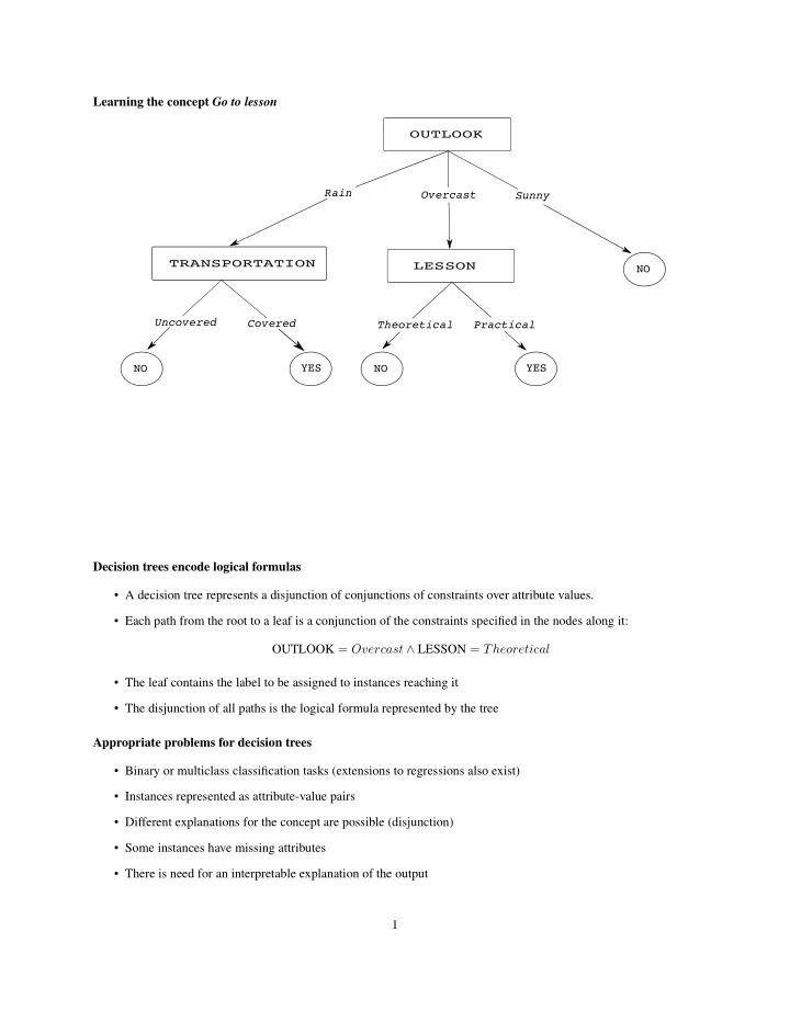
Learning the concept Go to lesson

OUTLOOK LESSON TRANSPORTATION

Rain Overcast Sunny Covered Uncovered Theoretical Practical NO YES YES NO NO

Decision trees encode logical formulas

• A decision tree represents a disjunction of conjunctions of constraints over attribute values.
• Each path from the root to a leaf is a conjunction of the constraints specified in the nodes along it:

OUTLOOK = Overcast ∧ LESSON = Theoretical

• The leaf contains the label to be assigned to instances reaching it
• The disjunction of all paths is the logical formula represented by the tree

Appropriate problems for decision trees

• Binary or multiclass classification tasks (extensions to regressions also exist)
• Instances represented as attribute-value pairs
• Different explanations for the concept are possible (disjunction)
• Some instances have missing attributes
• There is need for an interpretable explanation of the output

1

Learning decision trees

• Greedy top-down strategy (ID3 - Quinlan 1986, C4-5 - Quinlan 1993)
• For each node, starting from the root with full training set:
• 1. Choose best attribute to be evaluated
• 2. Add a child for each attribute value
• 3. Split node training set into children according to value of chosen attribute
• 4. Stop splitting a node if it contains examples from a single class, or there are no more attributes to test.
• Divide et impera approach

Chosing the best attribute Entropy

• A measure of the amount of information contained in a collection of instances S which can take a number c of

possible values. H(S) = −

c

• i=1

pilog2pi where pi is the fraction of S taking value i.

• In our case instances are training examples and values are class labels
• The entropy of a set of labelled examples measures its label inhomogeneity

Chosing the best attribute Information gain

• Expected reduction in entropy obtained by partitioning a set S according to the value of a certain attribute A

IG(S, A) = H(S) −

• v∈V alues(A)

|Sv| |S| H(Sv) where V alues(A) is the set of possible values taken by A and Sv is the subset of S taking value v at attribute A.

• The second term represents the sum of entropies of subsets of examples obtained partitioning over A values,

weighted by their respective sizes.

• An attribute with high information gain tends to produce homogeneous groups in terms of labels, thus favouring

their classification. 2

Issues in decision tree learning Overfitting avoidance

• Requiring that each leaf has only examples of a certain class can lead to very complex trees.
• A complex tree can easily overfit the training set, incorporating random regularities not representative of the full

distribution, or noise in the data.

• It is possible to accept impure leaves, assigning them the label of the majority of their training examples
• Two possible strategies to prune a decision tree:

pre-pruning decide whether to stop splitting a node even if it contains training examples with different labels. post-pruning learn a full tree and successively prune it removing subtrees. Reduced error pruning

• Post-pruning strategy
• Assumes a separate labelled validation set for the pruning stage.

The procedure

• 1. For each node in the tree:
• Evaluate the performance on the validation set when removing the subtree rooted at it
• 2. If all node removals worsen performance, STOP.
• 3. Choose the node whose removal has the best performance improvement
• 4. Replace the subtree rooted at it with a leaf
• 5. Assign to the leaf the majority label of all examples in the subtree
• 6. Return to 1

Issues in decision tree learning Dealing with continuous-valued attributes

• Continuous valued attributes need to be discretized in order to be used in internal nodes tests
• Discretization threshold can be chosen in order to maximize the attribute quality criterion (e.g. infogain)
• Procedure:
• 1. Examples are sorted according to their continuous attribute values
• 2. For each pair of successive examples having different labels, a candidate threshold is placed as the average
• f the two attribute values.
• 3. For each candidate threshold, the infogain achieved splitting examples according to it is computed
• 4. The threshold producing the higher infogain is used to discretize the attribute

3

Issues in decision tree learning Alternative attribute test measures

• The information gain criterion tends to prefer attributes with a large number of possible values
• As an extreme, the unique ID of each example is an attribute perfectly splitting the data into singletons, but it

will be of no use on new examples

• A measure of such spread is the entropy of the dataset wrt the attribute value instead of the class value:

HA(S) = −

• v∈V alues(A)

|Sv| |S| log2 |Sv| |S|

• The gain ratio measure downweights the information gain by such attribute value entropy

IGR(S, A) = IG(S, A) HA(S) Issues in decision tree learning Handling attributes with missing values

• Assume example x with class c(x) has missing value for attribute A.
• when attribute A is to be tested at node n:
• the complex solution implies that at test time, for each candidate class, all fractions of the test example which

reached a leaf with that class are summed, and the example is assigned the class with highest overall value Random forests Training

• 1. Given a training set of N examples, sample N examples with replacement (i.e. same example can be selected

multiple times)

• 2. Train a decision tree on the sample, selecting at each node m features at random among which to choose the

best one

• 3. Repeat steps 1 and 2 M times in order to generate a forest of M trees

Testing

• 1. Test the example with each tree in the forest
• 2. Return the majority class among the predictions

4