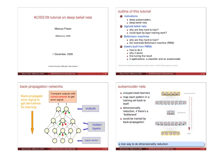
outline of this tutorial motivations 1 ACISS09 tutorial on deep - - PowerPoint PPT Presentation

ACISS’09 tutorial on deep belief nets

Marcus Frean

Melbourne, 2009

1 December, 2009

Victoria University, Wellington, New Zealand Marcus Frean (Melbourne, 2009) ACISS’09 tutorial on deep belief nets 1 / 60

• utline of this tutorial

1

motivations

deep autoencoders deep belief nets

2

sigmoid belief nets

why are they hard to train? could layer-by-layer training work?

3

Boltzmann machines

why are they hard to train? the restricted Boltzmann machine (RBM)

4

towers built from RBMs

how to do it why it works fine-tuning the result 2 applications: a classifier and an autoencoder

Several of the diagrams used here are based on those in Geoff Hinton’s papers & lectures. Marcus Frean (Melbourne, 2009) ACISS’09 tutorial on deep belief nets 2 / 60

back-propagation networks

Marcus Frean (Melbourne, 2009) ACISS’09 tutorial on deep belief nets 3 / 60

autoencoder nets

unsupervised learners map each pattern in a training set back to itself dimensionality reduction, if there’s a ”bottleneck” could be trained by back-propagation a nice way to do dimensionality reduction

Marcus Frean (Melbourne, 2009) ACISS’09 tutorial on deep belief nets 4 / 60

why haven’t deep auto-encoders worked?

all the hidden units interact the gradient gets tiny as you move away from the ”output” layer too hard to learn

Marcus Frean (Melbourne, 2009) ACISS’09 tutorial on deep belief nets 5 / 60

belief nets

A belief net is a directed acyclic graph composed of stochastic variables We get to observe some of the variables and would like to solve two problems:

1

The inference problem: Infer the states of unobserved variables

2

The learning problem: Adjust the interactions between variables to make the network more likely to generate the observed data.

Marcus Frean (Melbourne, 2009) ACISS’09 tutorial on deep belief nets 6 / 60

parameterized belief networks

Large belief nets are still too powerful to learn with finite data. But we can parameterize the factors: e.g. sigmoid function...

Marcus Frean (Melbourne, 2009) ACISS’09 tutorial on deep belief nets 7 / 60

what would a really interesting generative model for (say) images look like?

stochastic lots of units several layers easy to sample from sigmoid belief net an interesting generative model

Marcus Frean (Melbourne, 2009) ACISS’09 tutorial on deep belief nets 8 / 60

stochastic neurons

input to the ith neuron: φi =

• j

wjixj probability of generating a 1: pi = 1 1 + exp(φi) learning rule for making x more likely: ∆wji ∝ (xi − pi)xj it’s easy to make particular patterns more likely

Marcus Frean (Melbourne, 2009) ACISS’09 tutorial on deep belief nets 9 / 60

sampling from the joint

It is easy to sample from the prior p(x) = p(h, v) of a sigmoidal belief net: p(x) = p(x1, x2 . . . xn) =

• i

p(xi|parentsi) so we sample from each layer in turn, ending at the visible units. This seems like an attractive generative model.

Marcus Frean (Melbourne, 2009) ACISS’09 tutorial on deep belief nets 10 / 60

but...

to learn better weights based on a training set, we need to generate samples from the posterior, not the prior joint = p(h, v) = ”generative model”: start at the top and sample from sigmoids posterior = p(h|v) = ”recognition model”: sample from hidden units, given the visible ones. how to draw such samples? filter from the generative model?// no!

• h dear

Marcus Frean (Melbourne, 2009) ACISS’09 tutorial on deep belief nets 11 / 60

Gibbs sampling

To draw samples from p(x) = p(x1, x2, . . . , xn):

1

choose i at random

2

choose xi from p(xi|x\i)

adapted from David MacKay’s classic book

This results in a Markov Chain. Running the chain for long enough − → samples from p(x).

Marcus Frean (Melbourne, 2009) ACISS’09 tutorial on deep belief nets 12 / 60

Gibbs sampling in sigmoid belief nets

So what does p(xi|x\i) look like, in a sigmoid belief net? two hidden ”causes” visible node is observed... Gibbs sampling for h1, h2: p(h1 = 1|v = 1) =

• 1 + (1 − f(b1)) f(w2)

f(b1) f(w1 + w2) −1 = yuck! Gibbs sampler in sigmoid belief net: ugly, slow reason is ’explaining away’

Marcus Frean (Melbourne, 2009) ACISS’09 tutorial on deep belief nets 13 / 60

explaining away

Hidden states are independent in the prior dependent in the posterior That dependence means sampling from

• ne hidden unit has to cause a change

in how all other hidden units update their states. But we are interested in nets with lots of hidden units. an inconvenient truth: there’s no quick way to draw a sample from p(hidden|visible)

Marcus Frean (Melbourne, 2009) ACISS’09 tutorial on deep belief nets 14 / 60

sigmoidal belief nets are:

Easy to sample from as a generative model, but hard to learn

1

sampling from the posterior is slow, due to explaining away. This also makes them hard to use for recognition.

2

‘deep’ layers learn nothing until the ‘shallow’ ones have settled, but shallow layers have to learn while being driven by the deep layers (chicken and egg...) Let’s ignore the quibbles about slowness for a moment, and consider this idea: one way around the second difficulty might be to train the first layer as a simple BN first, and then the second layer, and so on.

Marcus Frean (Melbourne, 2009) ACISS’09 tutorial on deep belief nets 15 / 60

building a deep BN layer-by-layer

Here’s a way to train a multilayer sigmoid belief net:

1

start with a single layer only. The hidden units are driven by bias inputs only. Train to maximize the likelihood of generating the training data.

2

freeze the weights in that layer, and replace the hidden units’ bias inputs by a second layer of weights.

3

train the second layer of weights to maximize the likelihood.

4

and so on... Question: what should the training set be for the second layer?

Marcus Frean (Melbourne, 2009) ACISS’09 tutorial on deep belief nets 16 / 60

the EM algorithm

The W1 weights, and the biases into the hidden units, are trained so as to maximize the probability of generating the patterns on visible units in a data set. The EM algorithm achieves this by repeating two steps, for each v in the training data:

E step: calculate p(h|v) M step: move the W1 weights so as to make v more likely, under

p(h|v). And move the hidden biases to better produce that distribution.

Marcus Frean (Melbourne, 2009) ACISS’09 tutorial on deep belief nets 17 / 60

the EM algorithm, via sampling

In practice we can’t work with the posterior p(h|v) analytically: we have to sample from it instead. For each v in the training data:

E step: draw a sample from p(h|v) M step: move the W1 weights so as to make v more likely, given

that h. Move the hidden biases to better produce that h.

Marcus Frean (Melbourne, 2009) ACISS’09 tutorial on deep belief nets 18 / 60

aggregate posterior

Averaging over the training set, we have an aggregate posterior distribution: pagg(h) =

• v∈D

p(h|v) So the W1 weights end up at values that maximize the likelihood

• f the data, given h sampled from the aggregate posterior

distribution. The hidden bias weights end up at values that approximate this distribution.

Marcus Frean (Melbourne, 2009) ACISS’09 tutorial on deep belief nets 19 / 60

training the next layer

Q: what is the best thing that the second layer could learn to do? A: accurately generate the aggre- gate posterior distribution over the layer 1 hidden units. It is the distri- bution that makes the training data most likely, given W1 Easy! For each visible pattern, we just collect one sample (or more) from p(h|v). This gives us a greedy, layer-wise procedure for training deep belief nets.

Marcus Frean (Melbourne, 2009) ACISS’09 tutorial on deep belief nets 20 / 60

a comment about factorial distributions

This greedy procedure doesn’t work at all well. Subsequent layers add very little to what the first layer achieves, in modelling the data set. Why not? Consider some patterns v on a set of visible nodes. If these came from a world where the components of each vector are independent, then p(v) = p(v1, v2 . . . vn) =

• i

p(vi) and we say p(v) is factorial. If p(v) is factorial, there is no point in having hidden units in the gener- ative model ... a model that included hidden units could do no better than a model with just bias inputs to the visibles.

Marcus Frean (Melbourne, 2009) ACISS’09 tutorial on deep belief nets 21 / 60

why does greedy training fail for deep belief nets?

Consider the 1-layer architecture, and imagine going through the training set, clamping each visible pattern in turn, and generating a set

• f hidden patterns from the posterior p(h|v). These would be samples

from an “aggregate posterior”, namely pagg(h) ∝

• v∈D

p(h|v) Notice: The posterior p(h|v) is not factorial. The prior over h is factorial Given that, learning W1 weights with EM will result in weights that tend to make the aggregate posterior as factorial as possible. But a factorial aggregrate posterior is the very last thing we want for a greedy learning procedure, because it leaves nothing left for W2 to do!

Marcus Frean (Melbourne, 2009) ACISS’09 tutorial on deep belief nets 22 / 60

why does greedy training fail for deep belief nets?

EM:

1

for each v, sample from the posterior

2

make these v and h more likely under the joint prior distribution is factorial − → W1 tries to learn features that are independent in the prior but this is premature: we want to add another layer precisely because we DON’T BELIEVE THIS!

Marcus Frean (Melbourne, 2009) ACISS’09 tutorial on deep belief nets 23 / 60

Boltzmann machines

If we connect stochastic sigmoid units via symmetric weights, and avoid self-weights, we get a Boltzmann machine. A Boltzmann machine generates state x with probability p(x) ∝ e−E(x) where E is the energy E(x) = −1 2

• i,j

xixjwij −

• i

xibi In other words, Gibbs sampling for the above distribution is achieved by calculating the weighted sum into each unit, putting it through the sigmoid function, and choosing to output a 1 with the resulting probability. but you have to run a Markov Chain: it’s not ‘instant’.

Marcus Frean (Melbourne, 2009) ACISS’09 tutorial on deep belief nets 24 / 60

Gibbs sampling in Boltzmann machines

sampling from the joint: just use the sigmoid activation rule sampling from hiddens, given a visible pattern: just use the sigmoid activation rule i.e.... just use the sigmoid activation rule Contrast that with the sigmoid belief net, where sampling from the joint was easy and instant, but sampling from the posterior wasn’t (and didn’t use the sigmoid activation). sampling from a Boltzmann machine easy pretty (but requires waiting for a Markov chain to reach equilibrium)

Marcus Frean (Melbourne, 2009) ACISS’09 tutorial on deep belief nets 25 / 60

learning in Boltzmann machines

The log likelihood of generating the training set D is log L =

• v∈D

log p(v) where p(v) =

• all h

p(v, h) with p(v, h) = e−E(v,h) Z Z is normalisation, summed over all possible states. learning by gradient ascent ∆wij ∝

∂ ∂wij log L

Piece of cake, surely...

Marcus Frean (Melbourne, 2009) ACISS’09 tutorial on deep belief nets 26 / 60

learning in Boltzmann machines

The gradient turns out to be: ∂ ∂wij log P(D) = xi xjP data

x

− xi xjPx As a learning rule, this is: ∆wij = η

• xi xjP data

x

− xi xjPx

• (1)

learning in Boltzmann machines clamped phase: “clamp” each training pattern to the units, do Gibbs sampling on the hidden units, and accumulate the Hebbian changes. unclamped phase: do Gibbs sampling on all units, and accumulate anti-Hebbian changes.

Marcus Frean (Melbourne, 2009) ACISS’09 tutorial on deep belief nets 27 / 60

the problem

The gradient estimate is itself the difference between two noisy estimates, each of which requires sampling from a long MCMC chain, after waiting for it to reach equilibrium. This learning algorithm is beautiful but glacially slow in practice, to the point of being unusable. Despite their intuitive appeal as generative models, and their tempting similarities with biological neural nets, Boltzmann machines seemed doomed to the scrap heap until recently. We’re going to do two tricks to make Boltzmann machines practical devices:

1

restrict the connectivity.

2

use a new learning algorithm to train the weights. and then we’re going to show how to use them to solve the towers problem of sigmoid belief nets...

Marcus Frean (Melbourne, 2009) ACISS’09 tutorial on deep belief nets 28 / 60

trick # 1: restrict the connections

Assume visible units are one layer, and hidden units are another. Throw out all the connections within each layer. Restricted Boltzmann machine (RBM)

Marcus Frean (Melbourne, 2009) ACISS’09 tutorial on deep belief nets 29 / 60

Gibbs sampling in an RBM

Since none of the units in a layer are connected, we can do Gibbs sampling by updating all of one layer at a time. This is called “alternating” Gibbs sampling.

Marcus Frean (Melbourne, 2009) ACISS’09 tutorial on deep belief nets 30 / 60

learning in an RBM

The very first upward pass gives us a sample from the equilibrium distribution over hidden units, given the visible ones. The clamped Hebbian phase of BM learning is done in the first step! This is a consequence of the fact that, in the RBM graphical model, hidden activities are conditionally independent of one another given the visible activities. FAST The anti-Hebbian phase involves unclamping the inputs, and waiting long enough to get a sample from the generative

• distribution. SLOW.

Marcus Frean (Melbourne, 2009) ACISS’09 tutorial on deep belief nets 31 / 60

learning in an RBM

Repeat for all data:

1

start with a training vector on the visible units

2

then alternate between updating all the hidden units in parallel and updating all the visible units in parallel ∆wij = η

• vi hj0 − vi hj∞

restricted connectivity is trick #1: it saves waiting for equilibrium in the clamped phase.

Marcus Frean (Melbourne, 2009) ACISS’09 tutorial on deep belief nets 32 / 60

trick # 2: curtail the Markov chain during learning

1

start with a training vector on the visible units

2

update all the hidden units in parallel

3

update all the visible units in parallel to get a “reconstruction”

4

update the hidden units again ∆wij = η

• vi hj0 − vi hj1

This is not following the correct gradient, but works well in practice. Hinton calls this “learning by contrastive divergence”.

Marcus Frean (Melbourne, 2009) ACISS’09 tutorial on deep belief nets 33 / 60

why does this work?

If we start at a data point, the Markov chain wanders off towards patterns that are more likely. We can see the direction it is wandering in in just a few steps. It’s a big waste of time to let it go all the way to equilibrium. NOTE: in an RBM the hidden units are conditionally independent given the visible ones, so there is no “explaining away” inference required. trick #2: contrastive divergence this saves waiting for equilibrium in the unclamped phase.

Marcus Frean (Melbourne, 2009) ACISS’09 tutorial on deep belief nets 34 / 60

what kinds of distributions are RBMs well-suited for?

A single RBM and appropriate weights can generate any desired distribution over the visible units, if we give it enough hidden units (≈ 2# visible). The probability of the joint state in an RBM is P(v, h|W) ∝ exp(hTWv) and so P(v|W) ∝

• h

exp(hTWv)

Marcus Frean (Melbourne, 2009) ACISS’09 tutorial on deep belief nets 35 / 60

what kinds of distributions are RBMs well-suited for?

Carefully tracking terms (!), in log space this leads to: log P(v|W) = w0⋆

• biases

·v +

• j

log(1 + ewj⋆·v) + constant where wj⋆ is the vector of weights between the jth hidden unit and the visible units. a linear trend across the input space a sum of functions of form f = log(1 + eφ). This is zero for φ < 0 and the identity function for φ > 0, with a smooth transition. Each hidden unit represents a “feature” characterised by the direction

• f its weight vector wj⋆

The hidden unit lowers the energy of any states that are aligned with this vector, making them more likely.

Marcus Frean (Melbourne, 2009) ACISS’09 tutorial on deep belief nets 36 / 60

natural distributions for RBMs

RBMs seem predisposed to capture distributions consisting of conjunctions of high probability features. They should find it difficult to capture distributions that have ‘probability holes’ in them, since they can only add thresholded ramps together. To make a ‘hole’, they essentially have to add probability mass everywhere else. But this needs to be taken with a grain of salt. David MacKay and I trained RBMs (using the exact gradient) to learn “parity” distribution problems: exponentially many probability holes. Incredibly, an RBM with 6 hidden units can learn the parity distribution

• n 6 visible units perfectly! It does this by arranging a set of of 6 ramps

in just the right way to get high probability mass on all 32 of the desired patterns, while staying low for the 32 undesirable ones.

Marcus Frean (Melbourne, 2009) ACISS’09 tutorial on deep belief nets 37 / 60

an RBM with 6 hidden units doing 6 bit parity

Marcus Frean (Melbourne, 2009) ACISS’09 tutorial on deep belief nets 38 / 60

RBM summary

Two tricks were used to make Boltzmann machines practical devices: restrict the wiring This saves waiting for equi- librium in the clamped phase. truncate the Markov chain This saves waiting for equi- librium in the unclamped phase. (contrastive divergence)

Marcus Frean (Melbourne, 2009) ACISS’09 tutorial on deep belief nets 39 / 60

e.g. training data for a single class

Marcus Frean (Melbourne, 2009) ACISS’09 tutorial on deep belief nets 40 / 60

e.g. samples from an RBM trained on a single class

Marcus Frean (Melbourne, 2009) ACISS’09 tutorial on deep belief nets 41 / 60

e.g. weights after training on a single class

Marcus Frean (Melbourne, 2009) ACISS’09 tutorial on deep belief nets 42 / 60

a suggestion

greedy layer-wise learning take samples from the aggregate posterior and use them to train a another layer (and then another... and so on). To generate data, we could

1

run alternating Gibbs sampling for a while on the top layer, and then

2

do a top-down pass to the visible layer. This gives us a deep belief net (with an RBM as the top layer).

Marcus Frean (Melbourne, 2009) ACISS’09 tutorial on deep belief nets 43 / 60

a suggestion

But why would we expect this to do any better than the more obvious procedure of using single-layer sigmoid belief nets in the same way? Two ideas that help understanding:

1

RBMs are already deep BNs...

2

RBMs don’t try to force the aggregate posterior to be factorial...

Marcus Frean (Melbourne, 2009) ACISS’09 tutorial on deep belief nets 44 / 60

RBMs are already belief nets

an RBM with alternating Gibbs Sampling is equivalent to a sigmoid belief net with ∞ many layers. So when we train an RBM, we’re really training an ∞ deep belief net! It’s just that the weights of all layers are tied.

Marcus Frean (Melbourne, 2009) ACISS’09 tutorial on deep belief nets 45 / 60

RBMs don’t make the aggregate posterior ∼factorial

in a 1-layer sigmoid belief net: The prior over hiddens is factorial, but the posterior isn’t. Tries to make the aggregate posterior factorial. ...leaves little for subsequent layers to do. in a restricted Boltzmann machine: The posterior over hiddens is factorial, but the prior isn’t. DOESN’T try to force the aggregate posterior to be factorial. ...leaves more for the next layer to do.

Marcus Frean (Melbourne, 2009) ACISS’09 tutorial on deep belief nets 46 / 60

1 layer: weights and samples after training on “4”

Marcus Frean (Melbourne, 2009) ACISS’09 tutorial on deep belief nets 47 / 60

2 layer network

Marcus Frean (Melbourne, 2009) ACISS’09 tutorial on deep belief nets 48 / 60

training data for multiple classes

Marcus Frean (Melbourne, 2009) ACISS’09 tutorial on deep belief nets 49 / 60

weights after training on multiple classes

Marcus Frean (Melbourne, 2009) ACISS’09 tutorial on deep belief nets 50 / 60

samples from RBM trained on multiple classes

Marcus Frean (Melbourne, 2009) ACISS’09 tutorial on deep belief nets 51 / 60

application # 1: classification

Say there are 10 classes in the data. Since we have a generative model we can do semi-supervised learning: train the network almost entirely using unlabelled data, but include a “1-of-N” softmax unit in the top layer RBM. just use labels to identify which softmax state corresponds to which class label, at the end. Notice how different this is to supervised learning!

Marcus Frean (Melbourne, 2009) ACISS’09 tutorial on deep belief nets 52 / 60

application # 1: classification

(All details, and movies of the above in generative and recognition mode, are available via Geoff Hinton’s homepage) Marcus Frean (Melbourne, 2009) ACISS’09 tutorial on deep belief nets 53 / 60

fine tuning

So far, the up and down weights have been symmetric, as required by the Boltzmann machine learning algorithm. But once the tower is built they can be “untied”: wake: do a bottom-up pass, starting with a pattern from the training set. Use the delta rule to make this more likely under the generative model. sleep: do a top-down pass, starting from an equilibrium sample from the top RBM. Use the delta rule to make this more likely under the recognition model.

[CD version: start top RBM at the sample from the wake phase, and don’t wait for equilibrium before doing the top-down pass].

wake-sleep learning algorithm This unties the recognition weights from the generative ones.

Marcus Frean (Melbourne, 2009) ACISS’09 tutorial on deep belief nets 54 / 60

application # 2: autoencoding

basic training unrolling fine-tuning with back-prop Marcus Frean (Melbourne, 2009) ACISS’09 tutorial on deep belief nets 55 / 60

example: autoencoding digits

Notice: again, the fine tuning (by back-prop this time) achieves its effect by untying the generative and recognition weights.

Marcus Frean (Melbourne, 2009) ACISS’09 tutorial on deep belief nets 56 / 60

example: autoencoding digits

Codes for digits, produced by taking the first 2 principal components. Codes from a 784-1000-500-250-2 autoencoder.

Marcus Frean (Melbourne, 2009) ACISS’09 tutorial on deep belief nets 57 / 60

example: autoencoding documents

Hinton & Salakhutdinov, Science, 2007 Marcus Frean (Melbourne, 2009) ACISS’09 tutorial on deep belief nets 58 / 60

semantic hashing

Suppose the input is (say) word counts from documents Suppose the bottleneck is (say) 20 binary neurons Surprised? cf. 20 questions... That’s a 20-bit hashcode of the document It’s a “semantic” hash: similar documents will have similar codes We can navigate to documents that are “one question away” (without knowing what the question is..!)

Salakhutdinov & Hinton, 2007 Marcus Frean (Melbourne, 2009) ACISS’09 tutorial on deep belief nets 59 / 60

summary

1

Sigmoid belief nets

why are they hard to train? could layer-by-layer training work?

2

Boltzmann machines

why are they hard to train? RBMs

3

Deep belief nets built from RBMs

how to do it why it works fine-tuning the result [Key: untying the weights] 2 applications: a classifier and an autoencoder

I hope that helps - thanks for listening!

Marcus Frean (Melbourne, 2009) ACISS’09 tutorial on deep belief nets 60 / 60