Outline Notes: Riemann problems and phase plane (on board) - PDF document

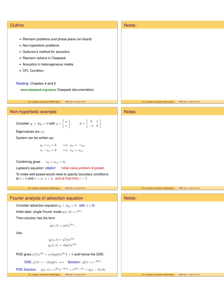
Outline Notes: • Riemann problems and phase plane (on board) • Non-hyperbolic problems • Godunov’s method for acoustics • Riemann solvers in Clawpack • Acoustics in heterogeneous media • CFL Condition Reading: Chapters 4 and 5 www.clawpack.org/users Clawpack documentation R.J. LeVeque, University of Washington IPDE 2011, June 24, 2011 R.J. LeVeque, University of Washington IPDE 2011, June 24, 2011 Non-hyperbolic example Notes: � u � � 0 1 � Consider q t + Aq x = 0 with q = , A = . v − 1 0 Eigenvalues are ± i . System can be written as: u t + v x = 0 = ⇒ u tt = − v xt v t − u x = 0 = ⇒ v xt = u xx u tt + u xx = 0 . Combining gives Laplace’s equation: elliptic! Initial value problem ill-posed. To make well-posed would need to specify boundary conditions at t = 0 and x = a, x = b , and at final time t = T . R.J. LeVeque, University of Washington IPDE 2011, June 24, 2011 R.J. LeVeque, University of Washington IPDE 2011, June 24, 2011 Fourier analysis of advection equation Notes: Consider advection equation q t + λq x = 0 with λ ∈ lR . Initial data: single Fourer mode q ( x, 0) = e ikx . Then solution has the form q ( x, t ) = g ( t ) e ikx . Use q t ( x, t ) = g ′ ( t ) e ikx q x ( x, t ) = ikg ( t ) e ikx PDE gives g ′ ( t ) e ikx + u � ikg ( t ) e ikx � = 0 and hence the ODE: ODE: g ′ ( t ) = − ikλg ( t ) = Solution: g ( t ) = e − ikλt ⇒ q ( x, t ) = e ikx e − ikλt = e ik ( x − λt ) = q ( x − λt, 0) . PDE Solution: R.J. LeVeque, University of Washington IPDE 2011, June 24, 2011 R.J. LeVeque, University of Washington IPDE 2011, June 24, 2011

Fourier analysis if λ complex Notes: Consider equation q t + λq x = 0 with λ = α + iβ with β > 0 . ( A real = ⇒ complex eigenvalues come in conjugate pairs.) Initial data: single Fourer mode q ( x, 0) = e ikx . As before, solution is just q ( x, t ) = e − ikλt e ikx . But now this is: q ( x, t ) = e − ik ( α + iβ ) t e ikx = e kβt e ik ( x − αt ) Translates at speed α but also grows exponentially in time. k can be arbitrarily large = ⇒ ill-posed problem. R.J. LeVeque, University of Washington IPDE 2011, June 24, 2011 R.J. LeVeque, University of Washington IPDE 2011, June 24, 2011 Finite differences vs. finite volumes Notes: Finite difference Methods • Pointwise values Q n i ≈ q ( x i , t n ) • Approximate derivatives by finite differences • Assumes smoothness Finite volume Methods � x i +1 / 2 1 • Approximate cell averages: Q n i ≈ q ( x, t n ) dx ∆ x x i − 1 / 2 • Integral form of conservation law, � x i +1 / 2 ∂ q ( x, t ) dx = f ( q ( x i − 1 / 2 , t )) − f ( q ( x i +1 / 2 , t )) ∂t x i − 1 / 2 leads to conservation law q t + f x = 0 but also directly to numerical method. R.J. LeVeque, University of Washington IPDE 2011, June 24, 2011 [FVMHP Chap. 4] R.J. LeVeque, University of Washington IPDE 2011, June 24, 2011 [FVMHP Chap. 4] Godunov’s Method for q t + f ( q ) x = 0 Notes: 1. Solve Riemann problems at all interfaces, yielding waves W p i − 1 / 2 and speeds s p i − 1 / 2 , for p = 1 , 2 , . . . , m . Riemann problem: Original equation with piecewise constant data. R.J. LeVeque, University of Washington IPDE 2011, June 24, 2011 [FVMHP Sec. 4.10] R.J. LeVeque, University of Washington IPDE 2011, June 24, 2011 [FVMHP Sec. 4.10]

Godunov’s Method for q t + f ( q ) x = 0 Notes: Then either: 1. Compute new cell averages by integrating over cell at t n +1 , 2. Compute fluxes at interfaces and flux-difference: i − ∆ t Q n +1 = Q n ∆ x [ F n i +1 / 2 − F n i − 1 / 2 ] i 3. Update cell averages by contributions from all waves entering cell: i − ∆ t Q n +1 = Q n ∆ x [ A + ∆ Q i − 1 / 2 + A − ∆ Q i +1 / 2 ] i m � ( s p i − 1 / 2 ) ± W p where A ± ∆ Q i − 1 / 2 = i − 1 / 2 . i =1 R.J. LeVeque, University of Washington IPDE 2011, June 24, 2011 [FVMHP Sec. 4.10] R.J. LeVeque, University of Washington IPDE 2011, June 24, 2011 [FVMHP Sec. 4.10] First-order REA Algorithm Notes: q n ( x, t n ) 1 Reconstruct a piecewise constant function ˜ defined for all x , from the cell averages Q n i . q n ( x, t n ) = Q n ˜ for all x ∈ C i . i 2 Evolve the hyperbolic equation exactly (or approximately) q n ( x, t n +1 ) a time ∆ t later. with this initial data to obtain ˜ 3 Average this function over each grid cell to obtain new cell averages 1 � Q n +1 q n ( x, t n +1 ) dx. = ˜ i ∆ x C i R.J. LeVeque, University of Washington IPDE 2011, June 24, 2011 [FVMHP Sec. 4.10] R.J. LeVeque, University of Washington IPDE 2011, June 24, 2011 [FVMHP Sec. 4.10] Godunov’s method for advection Notes: Q n i defines a piecewise constant function q n ( x, t n ) = Q n ˜ for x i − 1 / 2 < x < x i +1 / 2 i Discontinuities at cell interfaces = ⇒ Riemann problems. u > 0 u < 0 t n +1 t n +1 W i − 1 / 2 W i − 1 / 2 t n t n x i +1 / 2 x i +1 / 2 x i − 1 / 2 x i − 1 / 2 Q n Q n i − 1 i − 1 Q n Q n i i Q n Q n i +1 i +1 R.J. LeVeque, University of Washington IPDE 2011, June 24, 2011 [FVMHP Sec. 4.11] R.J. LeVeque, University of Washington IPDE 2011, June 24, 2011 [FVMHP Sec. 4.11]

First-order REA Algorithm Notes: Cell averages and piecewise constant reconstruction: After evolution: R.J. LeVeque, University of Washington IPDE 2011, June 24, 2011 [FVMHP Sec. 4.11] R.J. LeVeque, University of Washington IPDE 2011, June 24, 2011 [FVMHP Sec. 4.11] Cell update Notes: The cell average is modified by u ∆ t · ( Q n i − 1 − Q n i ) ∆ x So we obtain the upwind method i − u ∆ t Q n +1 = Q n ∆ x ( Q n i − Q n i − 1 ) . i R.J. LeVeque, University of Washington IPDE 2011, June 24, 2011 [FVMHP Sec. 4.11] R.J. LeVeque, University of Washington IPDE 2011, June 24, 2011 [FVMHP Sec. 4.11] Upwind for advection as a finite volume method Notes: i − ∆ t Q n +1 = Q n ∆ x ( F n i +1 / 2 − F n i − 1 / 2 ) i Advection equation: f ( q ) = uq � t n +1 F i − 1 / 2 ≈ 1 uq ( x i − 1 / 2 , t ) dt. ∆ t t n First order upwind: F i − 1 / 2 = u + Q n i − 1 + u − Q n i i − ∆ t Q n +1 = Q n ∆ x ( u + ( Q n i − Q n i − 1 ) + u − ( Q n i +1 − Q n i )) . i where u + = max( u, 0) , u − = min( u, 0) . R.J. LeVeque, University of Washington IPDE 2011, June 24, 2011 [FVMHP Sec. 4.1] R.J. LeVeque, University of Washington IPDE 2011, June 24, 2011 [FVMHP Sec. 4.1]

Godunov’s method Notes: Q n i defines a piecewise constant function q n ( x, t n ) = Q n ˜ for x i − 1 / 2 < x < x i +1 / 2 i Discontinuities at cell interfaces = ⇒ Riemann problems. Q n +1 i t n +1 t n Q n i | ( Q i − 1 , Q i ) q n ( x i − 1 / 2 , t ) ≡ q ∨ ˜ for t > t n . � t n +1 i − 1 / 2 = 1 | ( Q n | ( Q n F n f ( q ∨ i − 1 , Q n i )) dt = f ( q ∨ i − 1 , Q n i )) . ∆ t t n R.J. LeVeque, University of Washington IPDE 2011, June 24, 2011 [FVMHP Sec. 4.11] R.J. LeVeque, University of Washington IPDE 2011, June 24, 2011 [FVMHP Sec. 4.11] Wave-propagation viewpoint Notes: For linear system q t + Aq x = 0 , the Riemann solution consists of waves W p propagating at constant speed λ p . λ 2 ∆ t W 2 i − 1 / 2 W 1 W 1 i +1 / 2 i − 1 / 2 W 3 i − 1 / 2 m m i − 1 / 2 r p ≡ α p W p � � Q i − Q i − 1 = i − 1 / 2 . p =1 p =1 i − ∆ t Q n +1 = Q n λ 2 W 2 i − 1 / 2 + λ 3 W 3 i − 1 / 2 + λ 1 W 1 � � . i i +1 / 2 ∆ x R.J. LeVeque, University of Washington IPDE 2011, June 24, 2011 [FVMHP Sec. 3.8] R.J. LeVeque, University of Washington IPDE 2011, June 24, 2011 [FVMHP Sec. 3.8] Upwind wave-propagation algorithm Notes:   m m i − ∆ t Q n +1 = Q n � ( λ p ) + W p � ( λ p ) − W p i − 1 / 2 + i  i +1 / 2  ∆ x p =1 p =1 or i − ∆ t Q n +1 = Q n A + ∆ Q i − 1 / 2 + A − ∆ Q i +1 / 2 � � . i ∆ x where the fluctuations are defined by m ( λ p ) − W p A − ∆ Q i − 1 / 2 = � i − 1 / 2 , left-going p =1 m A + ∆ Q i − 1 / 2 = � ( λ p ) + W p i − 1 / 2 , right-going p =1 R.J. LeVeque, University of Washington IPDE 2011, June 24, 2011 R.J. LeVeque, University of Washington IPDE 2011, June 24, 2011