Outline Notes: Scalar nonlinear conservation laws Shocks and - - PDF document

SLIDE 1

Outline

• Scalar nonlinear conservation laws
• Shocks and rarefaction waves
• Entropy conditions
• Finite volume methods
• Approximate Riemann solvers
• Lax-Wendroff Theorem

Reading: Chapter 11, 12

R.J. LeVeque, University of Washington IPDE 2011, July 1, 2011

Notes:

R.J. LeVeque, University of Washington IPDE 2011, July 1, 2011

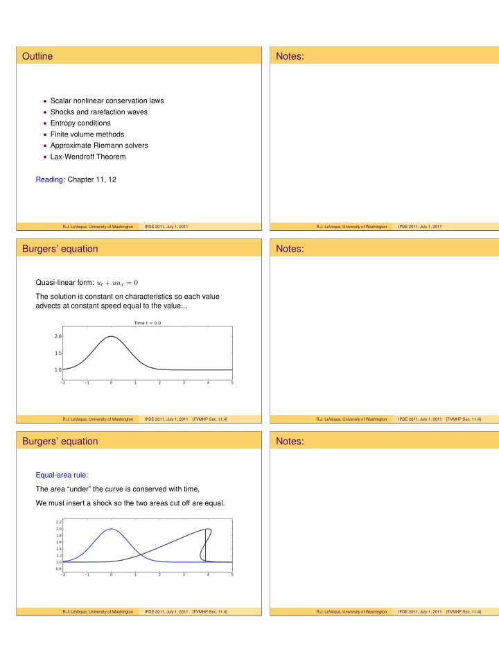
Burgers’ equation

Quasi-linear form: ut + uux = 0 The solution is constant on characteristics so each value advects at constant speed equal to the value...

R.J. LeVeque, University of Washington IPDE 2011, July 1, 2011 [FVMHP Sec. 11.4]

Notes:

R.J. LeVeque, University of Washington IPDE 2011, July 1, 2011 [FVMHP Sec. 11.4]

Burgers’ equation

Equal-area rule: The area “under” the curve is conserved with time, We must insert a shock so the two areas cut off are equal.

R.J. LeVeque, University of Washington IPDE 2011, July 1, 2011 [FVMHP Sec. 11.4]

Notes:

R.J. LeVeque, University of Washington IPDE 2011, July 1, 2011 [FVMHP Sec. 11.4]

SLIDE 2

Riemann problem for Burgers’ equation

ut + 1

2u2 x = 0,

ut + uux = 0. f(u) = 1

2u2,

f′(u) = u. Consider Riemann problem with states uℓ and ur. For any uℓ, ur, there is a weak solution consisting of this discontinuity propagating at speed given by the Rankine-Hugoniot jump condition: s =

1 2u2 r − 1 2u2 ℓ

ur − uℓ = 1 2(uℓ + ur). Note: Shock speed is average of characteristic speed on each side. This might not be the physically correct weak solution!

R.J. LeVeque, University of Washington IPDE 2011, July 1, 2011 [FVMHP Sec. 11.4]

Notes:

R.J. LeVeque, University of Washington IPDE 2011, July 1, 2011 [FVMHP Sec. 11.4]

Burgers’ equation

The solution is constant on characteristics so each value advects at constant speed equal to the value...

R.J. LeVeque, University of Washington IPDE 2011, July 1, 2011 [FVMHP Sec. 11.4]

Notes:

R.J. LeVeque, University of Washington IPDE 2011, July 1, 2011 [FVMHP Sec. 11.4]

Weak solutions to Burgers’ equation

ut + 1

2u2 x = 0,

uℓ = 1, ur = 2 Characteristic speed: u Rankine-Hugoniot speed: 1

2(uℓ + ur).

“Physically correct” rarefaction wave solution:

R.J. LeVeque, University of Washington IPDE 2011, July 1, 2011 [FVMHP Sec. 11.13 ]

Notes:

R.J. LeVeque, University of Washington IPDE 2011, July 1, 2011 [FVMHP Sec. 11.13 ]

SLIDE 3

Weak solutions to Burgers’ equation

ut + 1

2u2 x = 0,

uℓ = 1, ur = 2 Characteristic speed: u Rankine-Hugoniot speed: 1

2(uℓ + ur).

Entropy violating weak solution:

R.J. LeVeque, University of Washington IPDE 2011, July 1, 2011 [FVMHP Sec. 11.13 ]

Notes:

R.J. LeVeque, University of Washington IPDE 2011, July 1, 2011 [FVMHP Sec. 11.13 ]

Weak solutions to Burgers’ equation

ut + 1

2u2 x = 0,

uℓ = 1, ur = 2 Characteristic speed: u Rankine-Hugoniot speed: 1

2(uℓ + ur).

Another Entropy violating weak solution:

R.J. LeVeque, University of Washington IPDE 2011, July 1, 2011 [FVMHP Sec. 11.13 ]

Notes:

R.J. LeVeque, University of Washington IPDE 2011, July 1, 2011 [FVMHP Sec. 11.13 ]

Vanishing viscosity solution

We want q(x, t) to be the limit as ǫ → 0 of solution to qt + f(q)x = ǫqxx. This selects a unique weak solution:

• Shock if f′(ql) > f′(qr),
• Rarefaction if f′(ql) < f′(qr).

Lax Entropy Condition: A discontinuity propagating with speed s in the solution of a convex scalar conservation law is admissible only if f′(qℓ) > s > f′(qr), where s = (f(qr) − f(qℓ))/(qr − qℓ). Note: This means characteristics must approach shock from both sides as t advances, not move away from shock!

R.J. LeVeque, University of Washington IPDE 2011, July 1, 2011 [FVMHP Sec. 11.13 ]

Notes:

R.J. LeVeque, University of Washington IPDE 2011, July 1, 2011 [FVMHP Sec. 11.13 ]

SLIDE 4

Riemann problem for scalar nonlinear problem

qt + f(q)x = 0 with data q(x, 0) = ql if x < 0 qr if x ≥ 0 Piecewise constant with a single jump discontinuity. For Burgers’ or traffic flow with quadratic flux, the Riemann solution consists of:

• Shock wave if f′(ql) > f′(qr),
• Rarefaction wave if f′(ql) < f′(qr).

Five possible cases:

R.J. LeVeque, University of Washington IPDE 2011, July 1, 2011 [FVMHP Sec. 12.1]

Notes:

R.J. LeVeque, University of Washington IPDE 2011, July 1, 2011 [FVMHP Sec. 12.1]

Transonic rarefactions

Sonic point: us = 0 for Burgers’ since f′(0) = 0. Consider Riemann problem data uℓ = −0.5 < 0 < ur = 1.5. In this case wave should spread in both directions:

R.J. LeVeque, University of Washington IPDE 2011, July 1, 2011 [FVMHP Sec. 11.13 ]

Notes:

R.J. LeVeque, University of Washington IPDE 2011, July 1, 2011 [FVMHP Sec. 11.13 ]

Transonic rarefactions

Entropy-violating approximate Riemann solution: s = 1 2(uℓ + ur) = 0.5. Wave goes only to right, no update to cell average on left.

R.J. LeVeque, University of Washington IPDE 2011, July 1, 2011 [FVMHP Sec. 11.13 ]

Notes:

R.J. LeVeque, University of Washington IPDE 2011, July 1, 2011 [FVMHP Sec. 11.13 ]

SLIDE 5

Transonic rarefactions

If uℓ = −ur then Rankine-Hugoniot speed is 0: Similar solution will be observed with Godunov’s method if entropy-violating approximate Riemann solver used.

R.J. LeVeque, University of Washington IPDE 2011, July 1, 2011 [FVMHP Sec. 11.13 ]

Notes:

R.J. LeVeque, University of Washington IPDE 2011, July 1, 2011 [FVMHP Sec. 11.13 ]

Entropy-violating numerical solutions

Riemann problem for Burgers’ equation at t = 1 with uℓ = −1 and ur = 2:

−3 −2 −1 1 2 3 −1.5 −1 −0.5 0.5 1 1.5 2 2.5 Godunov with no entropy fix −3 −2 −1 1 2 3 −1.5 −1 −0.5 0.5 1 1.5 2 2.5 Godunov with entropy fix −3 −2 −1 1 2 3 −1.5 −1 −0.5 0.5 1 1.5 2 2.5 High−resolution with no entropy fix −3 −2 −1 1 2 3 −1.5 −1 −0.5 0.5 1 1.5 2 2.5 High−resolution with entropy fix

R.J. LeVeque, University of Washington IPDE 2011, July 1, 2011 [FVMHP Sec. 12.3]

Notes:

R.J. LeVeque, University of Washington IPDE 2011, July 1, 2011 [FVMHP Sec. 12.3]

Approximate Riemann solvers

For nonlinear problems, computing the exact solution to each Riemann problem may not be possible, or too expensive. Often the nonlinear problem qt + f(q)x = 0 is approximated by qt + Ai−1/2qx = 0, qℓ = Qi−1, qr = Qi for some choice of Ai−1/2 ≈ f′(q) based on data Qi−1, Qi. Solve linear system for αi−1/2: Qi − Qi−1 =

p αp i−1/2rp i−1/2.

Waves Wp

i−1/2 = αp i−1/2rp i−1/2 propagate with speeds sp i−1/2,

rp

i−1/2 are eigenvectors of Ai−1/2,

sp

i−1/2 are eigenvalues of Ai−1/2.

R.J. LeVeque, University of Washington IPDE 2011, July 1, 2011 [FVMHP Sec. 15.3.2 ]

Notes:

R.J. LeVeque, University of Washington IPDE 2011, July 1, 2011 [FVMHP Sec. 15.3.2 ]

SLIDE 6

Approximate Riemann solvers

qt + ˆ Ai−1/2qx = 0, qℓ = Qi−1, qr = Qi Often ˆ Ai−1/2 = f′(Qi−1/2) for some choice of Qi−1/2. In general ˆ Ai−1/2 = ˆ A(qℓ, qr). Roe conditions for consistency and conservation:

• ˆ

A(qℓ, qr) → f′(q∗) as qℓ, qr → q∗,

• ˆ

A diagonalizable with real eigenvalues,

• For conservation in wave-propagation form,

ˆ Ai−1/2(Qi − Qi−1) = f(Qi) − f(Qi−1).

R.J. LeVeque, University of Washington IPDE 2011, July 1, 2011 [FVMHP Sec. 15.3.2 ]

Notes:

R.J. LeVeque, University of Washington IPDE 2011, July 1, 2011 [FVMHP Sec. 15.3.2 ]

Approximate Riemann solvers

For a scalar problem, we can easily satisfy the Roe condition ˆ Ai−1/2(Qi − Qi−1) = f(Qi) − f(Qi−1). by choosing ˆ Ai−1/2 = f(Qi) − f(Qi−1) Qi − Qi−1 . Then r1

i−1/2 = 1 and s1 i−1/2 = ˆ

Ai−1/2 (scalar!). Note: This is the Rankine-Hugoniot shock speed. = ⇒ shock waves are correct, rarefactions replaced by entropy-violating shocks.

R.J. LeVeque, University of Washington IPDE 2011, July 1, 2011 [FVMHP Sec. 12.2 ]

Notes:

R.J. LeVeque, University of Washington IPDE 2011, July 1, 2011 [FVMHP Sec. 12.2 ]

Approximate Riemann solver

Qn+1

i

= Qn

i − ∆t

∆x

• A+∆Qi−1/2 + A−∆Qi+1/2
• .

For scalar advection m = 1, only one wave. Wi−1/2 = ∆Qi−1/2 = Qi − Qi−1 and si−1/2 = u, A−∆Qi−1/2 = s−

i−1/2Wi−1/2,

A+∆Qi−1/2 = s+

i−1/2Wi−1/2.

For scalar nonlinear: Use same formulas with Wi−1/2 = ∆Qi−1/2 and si−1/2 = ∆Fi−1/2/∆Qi−1/2. Need to modify these by an entropy fix in the trans-sonic rarefaction case.

R.J. LeVeque, University of Washington IPDE 2011, July 1, 2011 [FVMHP Sec. 12.3]

Notes:

R.J. LeVeque, University of Washington IPDE 2011, July 1, 2011 [FVMHP Sec. 12.3]

SLIDE 7

Entropy fix

Qn+1

i

= Qn

i − ∆t

∆x

• A+∆Qi−1/2 + A−∆Qi+1/2
• .

Revert to the formulas A−∆Qi−1/2 = f(qs) − f(Qi−1) left-going fluctuation A+∆Qi−1/2 = f(Qi) − f(qs) right-going fluctuation if f′(Qi−1) < 0 < f′(Qi). High-resolution method: still define wave W and speed s by Wi−1/2 = Qi − Qi−1, si−1/2 = (f(Qi) − f(Qi−1))/(Qi − Qi−1) if Qi−1 = Qi f′(Qi) if Qi−1 = Qi.

R.J. LeVeque, University of Washington IPDE 2011, July 1, 2011 [FVMHP Sec. 12.3]

Notes:

R.J. LeVeque, University of Washington IPDE 2011, July 1, 2011 [FVMHP Sec. 12.3]

Godunov flux for scalar problem

The Godunov flux function for the case f′′(q) > 0 is F n

i−1/2 =

   f(Qi−1) if Qi−1 > qs and s > 0 f(Qi) if Qi < qs and s < 0 f(qs) if Qi−1 < qs < Qi. =      min

Qi−1≤q≤Qi f(q)

if Qi−1 ≤ Qi max

Qi≤q≤Qi−1 f(q)

if Qi ≤ Qi−1, Here s = f(Qi)−f(Qi−1)

Qi−Qi−1

is the Rankine-Hugoniot shock speed.

R.J. LeVeque, University of Washington IPDE 2011, July 1, 2011 [FVMHP Sec. 12.1]

Notes:

R.J. LeVeque, University of Washington IPDE 2011, July 1, 2011 [FVMHP Sec. 12.1]

Entropy-violating numerical solutions

Riemann problem for Burgers’ equation at t = 1 with uℓ = −1 and ur = 2:

−3 −2 −1 1 2 3 −1.5 −1 −0.5 0.5 1 1.5 2 2.5 Godunov with no entropy fix −3 −2 −1 1 2 3 −1.5 −1 −0.5 0.5 1 1.5 2 2.5 Godunov with entropy fix −3 −2 −1 1 2 3 −1.5 −1 −0.5 0.5 1 1.5 2 2.5 High−resolution with no entropy fix −3 −2 −1 1 2 3 −1.5 −1 −0.5 0.5 1 1.5 2 2.5 High−resolution with entropy fix

R.J. LeVeque, University of Washington IPDE 2011, July 1, 2011 [FVMHP Sec. 12.3]

Notes:

R.J. LeVeque, University of Washington IPDE 2011, July 1, 2011 [FVMHP Sec. 12.3]

SLIDE 8

Entropy (admissibility) conditions

We generally require additional conditions on a weak solution to a conservation law, to pick out the unique solution that is physically relevant. In gas dynamics: entropy is constant along particle paths for smooth solutions, entropy can only increase as a particle goes through a shock. Entropy functions: Function of q that “behaves like” physical entropy for the conservation law being studied. NOTE: Mathematical entropy functions generally chosen to decrease for admissible solutions, increase for entropy-violating solutions.

R.J. LeVeque, University of Washington IPDE 2011, July 1, 2011 [FVMHP Sec. 11.4]

Notes:

R.J. LeVeque, University of Washington IPDE 2011, July 1, 2011 [FVMHP Sec. 11.4]

Entropy functions

A scalar-valued function η : lRm → lR is a convex function of q if the Hessian matrix η′′(q) with (i, j) element η′′

ij(q) =

∂2η ∂qi∂qj is positive definite for all q, i.e., satisfies vT η′′(q)v > 0 for all q, v ∈ lRm. Scalar case: reduces to η′′(q) > 0.

R.J. LeVeque, University of Washington IPDE 2011, July 1, 2011 [FVMHP Sec. 11.4]

Notes:

R.J. LeVeque, University of Washington IPDE 2011, July 1, 2011 [FVMHP Sec. 11.4]

Entropy functions

Entropy function: η : lRm → lR Entropy flux: ψ : lRm → lR chosen so that η(q) is convex and:

• η(q) is conserved wherever the solution is smooth,

η(q)t + ψ(q)x = 0.

• Entropy decreases across an admissible shock wave.

Weak form: x2

x1

η(q(x, t2)) dx ≤ x2

x1

η(q(x, t1)) dx + t2

t1

ψ(q(x1, t)) dt − t2

t1

ψ(q(x2, t)) dt with equality where solution is smooth.

R.J. LeVeque, University of Washington IPDE 2011, July 1, 2011 [FVMHP Sec. 11.4]

Notes:

R.J. LeVeque, University of Washington IPDE 2011, July 1, 2011 [FVMHP Sec. 11.4]

SLIDE 9

Entropy functions

How to find η and ψ satisfying this? η(q)t + ψ(q)x = 0 For smooth solutions gives η′(q)qt + ψ′(q)qx = 0. Since qt = −f′(q)qx this is satisfied provided ψ′(q) = η′(q)f′(q) Scalar: Can choose any convex η(q) and integrate. Example: Burgers’ equation, f′(u) = u and take η(u) = u2. Then ψ′(u) = 2u2 = ⇒ Entropy function: ψ(u) = 2

3u3.

R.J. LeVeque, University of Washington IPDE 2011, July 1, 2011 [FVMHP Sec. 11.4]

Notes:

R.J. LeVeque, University of Washington IPDE 2011, July 1, 2011 [FVMHP Sec. 11.4]

Weak solutions and entropy functions

The conservation laws ut + 1 2u2

• x

= 0 and

• u2

t +

2 3u3

• x

= 0 both have the same quasilinear form ut + uux = 0 but have different weak solutions, different shock speeds! Entropy function: η(u) = u2. A correct Burgers’ shock at speed s = 1

2(uℓ + ur) will have

total mass of η(u) decreasing.

R.J. LeVeque, University of Washington IPDE 2011, July 1, 2011 [FVMHP Sec. 11.4]

Notes:

R.J. LeVeque, University of Washington IPDE 2011, July 1, 2011 [FVMHP Sec. 11.4]

Entropy functions

x2

x1

η(q(x, t2)) dx ≤ x2

x1

η(q(x, t1)) dx + t2

t1

ψ(q(x1, t)) dt − t2

t1

ψ(q(x2, t)) dt

comes from considering the vanishing viscosity solution: qǫ

t + f(qǫ)x = ǫqǫ xx

Multiply by η′(qǫ) to obtain: η(qǫ)t + ψ(qǫ)x = ǫη′(qǫ)qǫ

xx.

Manipulate further to get η(qǫ)t + ψ(qǫ)x = ǫ

• η′(qǫ)qǫ

x

• x − ǫη′′(qǫ) (qǫ

x)2.

R.J. LeVeque, University of Washington IPDE 2011, July 1, 2011 [FVMHP Sec. 11.4]

Notes:

R.J. LeVeque, University of Washington IPDE 2011, July 1, 2011 [FVMHP Sec. 11.4]

SLIDE 10

Entropy functions

Smooth solution to viscous equation satisfies

η(qǫ)t + ψ(qǫ)x = ǫ

• η′(qǫ)qǫ

x

• x − ǫη′′(qǫ) (qǫ

x)2.

Integrating over rectangle [x1, x2] × [t1, t2] gives

x2

x1

η(qǫ(x, t2)) dx = x2

x1

η(qǫ(x, t1)) dx − t2

t1

ψ(qǫ(x2, t)) dt − t2

t1

ψ(qǫ(x1, t)) dt

• + ǫ

t2

t1

• η′(qǫ(x2, t)) qǫ

x(x2, t) − η′(qǫ(x1, t)) qǫ x(x1, t)

• dt

− ǫ t2

t1

x2

x1

η′′(qǫ) (qǫ

x)2 dx dt.

Let ǫ → 0 to get result: Term on third line goes to 0, Term of fourth line is always ≤ 0.

R.J. LeVeque, University of Washington IPDE 2011, July 1, 2011 [FVMHP Sec. 11.4]

Notes:

R.J. LeVeque, University of Washington IPDE 2011, July 1, 2011 [FVMHP Sec. 11.4]

Entropy functions

Weak form of entropy condition: ∞ ∞

−∞

• φtη(q) + φxψ(q)
• dx dt +

∞

−∞

φ(x, 0)η(q(x, 0)) dx ≥ 0 for all φ ∈ C1

0(l

R × lR) with φ(x, t) ≥ 0 for all x, t. Informally we may write η(q)t + ψ(q)x ≤ 0.

R.J. LeVeque, University of Washington IPDE 2011, July 1, 2011 [FVMHP Sec. 11.4]

Notes:

R.J. LeVeque, University of Washington IPDE 2011, July 1, 2011 [FVMHP Sec. 11.4]

Lax-Wendroff Theorem

Suppose the method is conservative and consistent with qt + f(q)x = 0, Fi−1/2 = F(Qi−1, Qi) with F(¯ q, ¯ q) = f(¯ q) and Lipschitz continuity of F. If a sequence of discrete approximations converge to a function q(x, t) as the grid is refined, then this function is a weak solution of the conservation law. Note: Does not guarantee a sequence converges (need stability). Two sequences might converge to different weak solutions. Also need to satisfy an entropy condition.

R.J. LeVeque, University of Washington IPDE 2011, July 1, 2011 [FVMHP Sec. 12.10]

Notes:

R.J. LeVeque, University of Washington IPDE 2011, July 1, 2011 [FVMHP Sec. 12.10]

SLIDE 11

Sketch of proof of Lax-Wendroff Theorem

Multiply the conservative numerical method Qn+1

i

= Qn

i − ∆t

∆x(F n

i+1/2 − F n i−1/2)

by Φn

i to obtain

Φn

i Qn+1 i

= Φn

i Qn i − ∆t

∆xΦn

i (F n i+1/2 − F n i−1/2).

This is true for all values of i and n on each grid. Now sum over all i and n ≥ 0 to obtain

∞

• n=0

∞

• i=−∞

Φn

i (Qn+1 i

−Qn

i ) = − ∆t

∆x

∞

• n=0

∞

• i=−∞

Φn

i (F n i+1/2 −F n i−1/2).

Use summation by parts to transfer differences to Φ terms.

R.J. LeVeque, University of Washington IPDE 2011, July 1, 2011 [FVMHP Sec. 12.10]

Notes:

R.J. LeVeque, University of Washington IPDE 2011, July 1, 2011 [FVMHP Sec. 12.10]

Sketch of proof of Lax-Wendroff Theorem

Obtain analog of weak form of conservation law: ∆x∆t ∞

• n=1

∞

• i=−∞

Φn

i − Φn−1 i

∆t

• Qn

i

+

∞

• n=0

∞

• i=−∞

Φn

i+1 − Φn i

∆x

• F n

i−1/2

• = −∆x

∞

• i=−∞

Φ0

i Q0 i .

Consider on a sequence of grids with ∆x, ∆t → 0. Show that any limiting function must satisfy weak form of conservation law.

R.J. LeVeque, University of Washington IPDE 2011, July 1, 2011 [FVMHP Sec. 12.10]

Notes:

R.J. LeVeque, University of Washington IPDE 2011, July 1, 2011 [FVMHP Sec. 12.10]

Analog of Lax-Wendroff proof for entropy

Show that the numerical flux function F leads to a numerical entropy flux Ψ such that the following discrete entropy inequality holds: η(Qn+1

i

) ≤ η(Qn

i ) − ∆t

∆x

• Ψn

i+1/2 − Ψn i−1/2

• .

Then multiply by test function Φn

i , sum and use summation by

parts to get discrete form of integral form of entropy condition. = ⇒ If numerical approximations converge to some function, then the limiting function satisfies the entropy condition.

R.J. LeVeque, University of Washington IPDE 2011, July 1, 2011 [FVMHP Sec. 12.11]

Notes:

R.J. LeVeque, University of Washington IPDE 2011, July 1, 2011 [FVMHP Sec. 12.11]

SLIDE 12

Entropy consistency of Godunov’s method

For Godunov’s method, F(Qi−1, Qi) = f(Q∨

|

i−1/2)

where Q∨

|

i−1/2 is the constant value

along xi−1/2 in the Riemann solution. Let Ψn

i−1/2 = ψ(Q∨

|

i−1/2)

Discrete entropy inequality follows from Jensen’s inequality: The value of η evaluated at the average value of ˜ qn is less than

• r equal to the average value of η(˜

qn), i.e., η

• 1

∆x xi+1/2

xi−1/2

˜ qn(x, tn+1) dx

• ≤

1 ∆x xi+1/2

xi−1/2

η

• ˜

qn(x, tn+1)

• dx.

R.J. LeVeque, University of Washington IPDE 2011, July 1, 2011 [FVMHP Sec. 12.11]

Notes:

R.J. LeVeque, University of Washington IPDE 2011, July 1, 2011 [FVMHP Sec. 12.11]