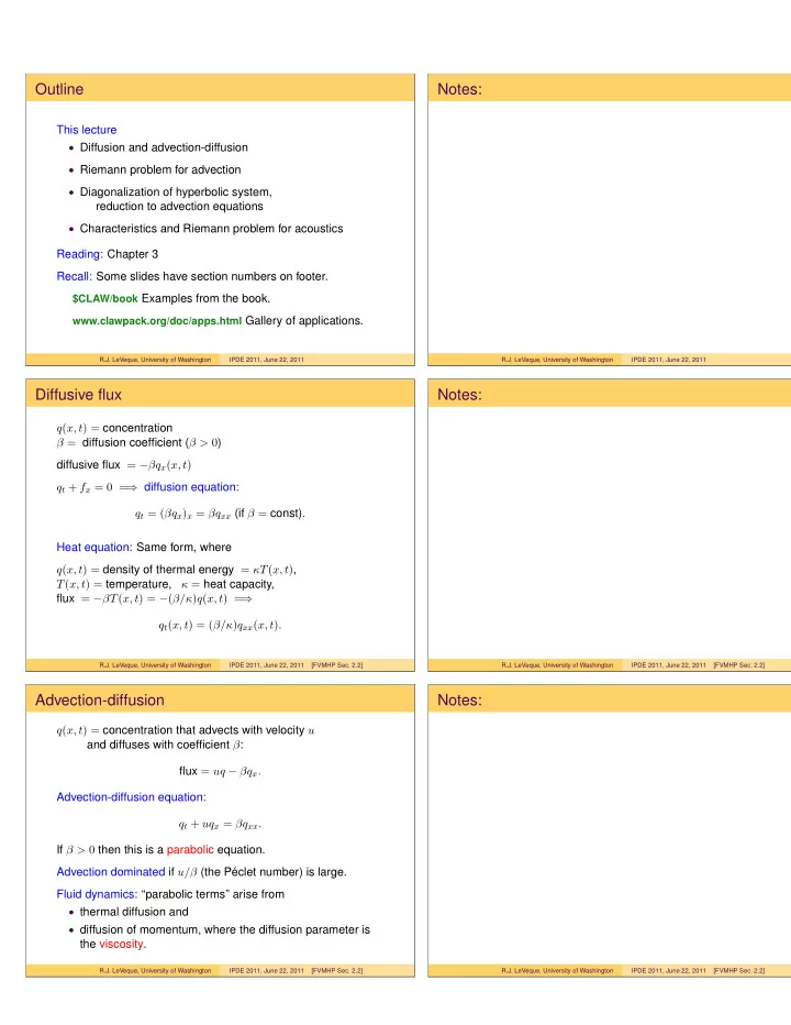
Outline Notes: This lecture Diffusion and advection-diffusion - - PDF document

SLIDE 1

Outline

This lecture

• Diffusion and advection-diffusion
• Riemann problem for advection
• Diagonalization of hyperbolic system,

reduction to advection equations

• Characteristics and Riemann problem for acoustics

Reading: Chapter 3 Recall: Some slides have section numbers on footer.

$CLAW/book Examples from the book. www.clawpack.org/doc/apps.html Gallery of applications.

R.J. LeVeque, University of Washington IPDE 2011, June 22, 2011

Notes:

R.J. LeVeque, University of Washington IPDE 2011, June 22, 2011

Diffusive flux

q(x, t) = concentration β = diffusion coefficient (β > 0) diffusive flux = −βqx(x, t) qt + fx = 0 = ⇒ diffusion equation: qt = (βqx)x = βqxx (if β = const). Heat equation: Same form, where q(x, t) = density of thermal energy = κT(x, t), T(x, t) = temperature, κ = heat capacity, flux = −βT(x, t) = −(β/κ)q(x, t) = ⇒ qt(x, t) = (β/κ)qxx(x, t).

R.J. LeVeque, University of Washington IPDE 2011, June 22, 2011 [FVMHP Sec. 2.2]

Notes:

R.J. LeVeque, University of Washington IPDE 2011, June 22, 2011 [FVMHP Sec. 2.2]

Advection-diffusion

q(x, t) = concentration that advects with velocity u and diffuses with coefficient β: flux = uq − βqx. Advection-diffusion equation: qt + uqx = βqxx. If β > 0 then this is a parabolic equation. Advection dominated if u/β (the Péclet number) is large. Fluid dynamics: “parabolic terms” arise from

• thermal diffusion and
• diffusion of momentum, where the diffusion parameter is

the viscosity.

R.J. LeVeque, University of Washington IPDE 2011, June 22, 2011 [FVMHP Sec. 2.2]

Notes:

R.J. LeVeque, University of Washington IPDE 2011, June 22, 2011 [FVMHP Sec. 2.2]

SLIDE 2

The Riemann problem

The Riemann problem consists of the hyperbolic equation under study together with initial data of the form q(x, 0) = ql if x < 0 qr if x ≥ 0 Piecewise constant with a single jump discontinuity from ql to qr. The Riemann problem is fundamental to understanding

• The mathematical theory of hyperbolic problems,
• Godunov-type finite volume methods

Why? Even for nonlinear systems of conservation laws, the Riemann problem can often be solved for general ql and qr, and consists of a set of waves propagating at constant speeds.

R.J. LeVeque, University of Washington IPDE 2011, June 22, 2011 [FVMHP Sec. 3.8]

Notes:

R.J. LeVeque, University of Washington IPDE 2011, June 22, 2011 [FVMHP Sec. 3.8]

The Riemann problem for advection

The Riemann problem for the advection equation qt + uqx = 0 with q(x, 0) = ql if x < 0 qr if x ≥ 0 has solution q(x, t) = q(x − ut, 0) = ql if x < ut qr if x ≥ ut consisting of a single wave of strength W1 = qr − ql propagating with speed s1 = u.

R.J. LeVeque, University of Washington IPDE 2011, June 22, 2011 [FVMHP Sec. 3.8]

Notes:

R.J. LeVeque, University of Washington IPDE 2011, June 22, 2011 [FVMHP Sec. 3.8]

Riemann solution for advection

q(x, T) x–t plane q(x, 0)

R.J. LeVeque, University of Washington IPDE 2011, June 22, 2011 [FVMHP Sec. 3.8]

Notes:

R.J. LeVeque, University of Washington IPDE 2011, June 22, 2011 [FVMHP Sec. 3.8]

SLIDE 3

Discontinuous solutions

Note: The Riemann solution is not a classical solution of the PDE qt + uqx = 0, since qt and qx blow up at the discontinuity. Integral form:

d dt x2

x1

q(x, t) dx = uq(x1, t) − uq(x2, t)

Integrate in time from t1 to t2 to obtain x2

x1

q(x, t2) dx − x2

x1

q(x, t1) dx = t2

t1

uq(x1, t) dt − t2

t1

uq(x2, t) dt. The Riemann solution satisfies the given initial conditions and this integral form for all x2 > x1 and t2 > t1 ≥ 0.

R.J. LeVeque, University of Washington IPDE 2011, June 22, 2011 [FVMHP Sec. 3.7]

Notes:

R.J. LeVeque, University of Washington IPDE 2011, June 22, 2011 [FVMHP Sec. 3.7]

Discontinuous solutions

Vanishing Viscosity solution: The Riemann solution q(x, t) is the limit as ǫ → 0 of the solution qǫ(x, t) of the parabolic advection-diffusion equation qt + uqx = ǫqxx. For any ǫ > 0 this has a classical smooth solution:

R.J. LeVeque, University of Washington IPDE 2011, June 22, 2011 [FVMHP Sec. 11.6]

Notes:

R.J. LeVeque, University of Washington IPDE 2011, June 22, 2011 [FVMHP Sec. 11.6]

Diagonalization of linear system

Consider constant coefficient linear system qt + Aqx = 0. Suppose hyperbolic:

• Real eigenvalues λ1 ≤ λ2 ≤ · · · ≤ λm,
• Linearly independent eigenvalues r1, r2, . . . , rm.

Let R = [r1|r2| · · · |rm] m × m matrix of eigenvectors. Then Arp = λprp means that AR = RΛ where Λ =      λ1 λ2 ... λm      ≡ diag(λ1, λ2, . . . , λm). AR = RΛ = ⇒ A = RΛR−1 and R−1AR = Λ. Similarity transformation with R diagonalizes A.

R.J. LeVeque, University of Washington IPDE 2011, June 22, 2011 [FVMHP Sec. 2.9]

Notes:

R.J. LeVeque, University of Washington IPDE 2011, June 22, 2011 [FVMHP Sec. 2.9]

SLIDE 4

Diagonalization of linear system

Consider constant coefficient linear system qt + Aqx = 0. Multiply system by R−1: R−1qt(x, t) + R−1Aqx(x, t) = 0. Introduce RR−1 = I: R−1qt(x, t) + R−1ARR−1qx(x, t) = 0. Use R−1AR = Λ and define w(x, t) = R−1q(x, t): wt(x, t) + Λwx(x, t) = 0. Since R is constant! This decouples to m independent scalar advection equations: wp

t (x, t) + λpwp x(x, t) = 0.

p = 1, 2, . . . , m.

R.J. LeVeque, University of Washington IPDE 2011, June 22, 2011 [FVMHP Sec. 2.9, 3.1]

Notes:

R.J. LeVeque, University of Washington IPDE 2011, June 22, 2011 [FVMHP Sec. 2.9, 3.1]

Solution to Cauchy problem

Suppose q(x, 0) = q

• (x)

for − ∞ < x < ∞. From this initial data we can compute data w

• (x) ≡ R−1q
• (x)

The solution to the decoupled equation wp

t + λpwp x = 0 is

wp(x, t) = wp(x − λpt, 0) = w

• p(x − λpt).

Putting these together in vector gives w(x, t) and finally q(x, t) = Rw(x, t). We can rewrite this as q(x, t) =

m

• p=1

wp(x, t) rp =

m

• p=1

w

• p(x − λpt) rp

R.J. LeVeque, University of Washington IPDE 2011, June 22, 2011 [FVMHP Sec. 3.1]

Notes:

R.J. LeVeque, University of Washington IPDE 2011, June 22, 2011 [FVMHP Sec. 3.1]

Linear acoustics

Example: Linear acoustics in a 1d gas tube q = p u

• p(x, t) = pressure perturbation

u(x, t) = velocity Equations: pt + κux = 0 Change in pressure due to compression ρut + px = 0 Newton’s second law, F = ma where K = bulk modulus, and ρ = unperturbed density of gas. Hyperbolic system: p u

• t

+

• κ

1/ρ p u

• x

= 0.

R.J. LeVeque, University of Washington IPDE 2011, June 22, 2011 [FVMHP Sec. 3.9.1]

Notes:

R.J. LeVeque, University of Washington IPDE 2011, June 22, 2011 [FVMHP Sec. 3.9.1]

SLIDE 5

Eigenvectors for acoustics

A =

• u0

K0 1/ρ0 u0

• (acoustics relative to

flow with speed u0) Eigenvectors: r1 = −ρ0c0 1

• ,

r2 = ρ0c0 1

• .

Check that Arp = λprp, where λ1 = u0 − c0, λ2 = u0 + c0. with c0 =

• K0/ρ0 =

⇒ K0 = ρ0c2

0.

Note: Eigenvectors are independent of u0. Let Z0 = ρ0c0 = √K0ρ0 = impedance.

R.J. LeVeque, University of Washington IPDE 2011, June 22, 2011 [FVMHP Sec. 2.8]

Notes:

R.J. LeVeque, University of Washington IPDE 2011, June 22, 2011 [FVMHP Sec. 2.8]

Physical meaning of eigenvectors

Eigenvectors for acoustics: r1 = −ρ0c0 1

• =

−Z0 1

• ,

r2 = ρ0c0 1

• =

Z0 1

• .

Consider a pure 1-wave (simple wave), at speed λ1 = −c0, If q

• (x) = ¯

q + w

• 1(x)r1 then

q(x, t) = ¯ q + w

• 1(x − λ1t)r1

Variation of q, as measured by qx or ∆q = q(x + ∆x) − q(x) is proportional to eigenvector r1, e.g. qx(x, t) = w

• 1

x(x − λ1t)r1

R.J. LeVeque, University of Washington IPDE 2011, June 22, 2011 [FVMHP Sec. 3.4, 3.5]

Notes:

R.J. LeVeque, University of Washington IPDE 2011, June 22, 2011 [FVMHP Sec. 3.4, 3.5]

Physical meaning of eigenvectors

Eigenvectors for acoustics: r1 = −ρ0c0 1

• =

−Z0 1

• ,

r2 = ρ0c0 1

• =

Z0 1

• .

In a simple 1-wave (propagating at speed λ1 = −c0), px ux

• = β(x)

−Z0 1

• The pressure variation is −Z0 times the velocity variation.

Similarly, in a simple 2-wave (λ2 = c0), px ux

• = β(x)

Z0 1

• The pressure variation is Z0 times the velocity variation.

R.J. LeVeque, University of Washington IPDE 2011, June 22, 2011 [FVMHP Sec. 3.5]

Notes:

R.J. LeVeque, University of Washington IPDE 2011, June 22, 2011 [FVMHP Sec. 3.5]

SLIDE 6

Acoustic waves

q(x, 0) =

• p
• (x)
• =

−p

• (x)

2Z0

−Z0 1

• +

p

• (x)

2Z0

Z0 1

• =

w1(x, 0)r1 + w2(x, 0)r2 =

• p
• (x)/2

−p

• (x)/(2Z0)
• +
• p
• (x)/2

p

• (x)/(2Z0)
• .

R.J. LeVeque, University of Washington IPDE 2011, June 22, 2011 [FVMHP Sec. 3.5]

Notes:

R.J. LeVeque, University of Washington IPDE 2011, June 22, 2011 [FVMHP Sec. 3.5]

Solution by tracing back on characteristics

The general solution for acoustics: q(x, t) = w1(x − λ1t, 0)r1 + w2(x − λ2t, 0)r2 = w1(x + c0t, 0)r1 + w2(x − c0t, 0)r2 Recall that w(x, 0) = R−1q(x, 0), i.e. w1(x, 0) = ℓ1q(x, 0), w2(x, 0) = ℓ2q(x, 0) where ℓ1 and ℓ2 are rows of R−1. R−1 = ℓ1 ℓ2

• Note: ℓ1 and ℓ2 are left-eigenvectors of A:

ℓpA = λpℓp since R−1A = ΛR−1.

R.J. LeVeque, University of Washington IPDE 2011, June 22, 2011 [FVMHP Sec. 3.5]

Notes:

R.J. LeVeque, University of Washington IPDE 2011, June 22, 2011 [FVMHP Sec. 3.5]

Solution by tracing back on characteristics

The general solution for acoustics: q(x, t) = w1(x − λ1t, 0)r1 + w2(x − λ2t, 0)r2 = w1(x + c0t, 0)r1 + w2(x − c0t, 0)r2

(x, t) x − λ2t = x − c0t x − λ1t = x + c0t

R.J. LeVeque, University of Washington IPDE 2011, June 22, 2011 [FVMHP Sec. 3.6]

Notes:

R.J. LeVeque, University of Washington IPDE 2011, June 22, 2011 [FVMHP Sec. 3.6]

SLIDE 7

Solution by tracing back on characteristics

The general solution for acoustics: q(x, t) = w1(x − λ1t, 0)r1 + w2(x − λ2t, 0)r2

q(x, t) w2(x − λ2t, 0) = ℓ2q(x − λ2t, 0) w1(x − λ1t, 0) = ℓ1q(x − λ1t, 0)

w2 constant w1 constant

R.J. LeVeque, University of Washington IPDE 2011, June 22, 2011 [FVMHP Sec. 3.5]

Notes:

R.J. LeVeque, University of Washington IPDE 2011, June 22, 2011 [FVMHP Sec. 3.5]

Riemann Problem

Special initial data: q(x, 0) = ql if x < 0 qr if x > 0 Example: Acoustics with bursting diaphram (ul = ur = 0) Pressure: Acoustic waves propagate with speeds ±c.

R.J. LeVeque, University of Washington IPDE 2011, June 22, 2011 [FVMHP Sec. 3.9.1]

Notes:

R.J. LeVeque, University of Washington IPDE 2011, June 22, 2011 [FVMHP Sec. 3.9.1]

Riemann Problem for acoustics

Waves propagating in x–t space: Left-going wave W1 = qm − ql and right-going wave W2 = qr − qm are eigenvectors of A.

R.J. LeVeque, University of Washington IPDE 2011, June 22, 2011 [FVMHP Sec. 3.8]

Notes:

R.J. LeVeque, University of Washington IPDE 2011, June 22, 2011 [FVMHP Sec. 3.8]

SLIDE 8

Riemann Problem for acoustics

In x–t plane: q(x, t) = w1(x + ct, 0)r1 + w2(x − ct, 0)r2 Decompose ql and qr into eigenvectors: ql = w1

l r1 + w2 l r2

qr = w1

rr1 + w2 rr2

Then qm = w1

rr1 + w2 l r2

R.J. LeVeque, University of Washington IPDE 2011, June 22, 2011 [FVMHP Sec. 3.9]

Notes:

R.J. LeVeque, University of Washington IPDE 2011, June 22, 2011 [FVMHP Sec. 3.9]

Riemann Problem for acoustics

ql = w1

l r1 + w2 l r2

qr = w1

rr1 + w2 rr2

Then qm = w1

rr1 + w2 l r2

So the waves W1 and W2 are eigenvectors of A: W1 = qm − ql = (w1

r − w1 l )r1

W2 = qr − qm = (w2

r − w2 l )r2.

R.J. LeVeque, University of Washington IPDE 2011, June 22, 2011 [FVMHP Sec. 3.9]

Notes:

R.J. LeVeque, University of Washington IPDE 2011, June 22, 2011 [FVMHP Sec. 3.9]

Riemann solution for a linear system

Linear hyperbolic system: qt + Aqx = 0 with A = RΛR−1. General Riemann problem data ql, qr ∈ lRm. Decompose jump in q into eigenvectors: qr − ql =

m

• p=1

αprp Note: the vector α of eigen-coefficients is α = R−1(qr − ql) = R−1qr − R−1ql = wr − wl. Riemann solution consists of m waves Wp ∈ lRm: Wp = αprp, propagating with speed sp = λp.

R.J. LeVeque, University of Washington IPDE 2011, June 22, 2011 [FVMHP Sec. 3.9]

Notes:

R.J. LeVeque, University of Washington IPDE 2011, June 22, 2011 [FVMHP Sec. 3.9]