Outline Notes: Godunovs method for acoustics Riemann solvers in - - PDF document

SLIDE 1

Outline

• Godunov’s method for acoustics
• Riemann solvers in Clawpack
• Acoustics in heterogeneous media
• CFL Condition
• Intro to Python plotting tools

Reading: Chapters 4 – 6

www.clawpack.org/users Clawpack documentation www.clawpack.org/users/plotting.html Plotting hints

See also Python and plotting sections of AMath 583 notes at

http://www.amath.washington.edu/~rjl/uwamath583s11

R.J. LeVeque, University of Washington IPDE 2011, June 27, 2011

Notes:

R.J. LeVeque, University of Washington IPDE 2011, June 27, 2011

Godunov (upwind) on acoustics

tn tn+1 Qn

i

Qn+1

i

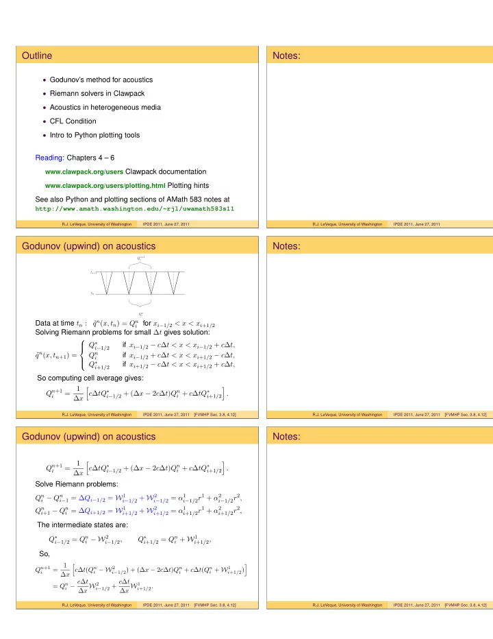
Data at time tn : ˜ qn(x, tn) = Qn

i

for xi−1/2 < x < xi+1/2 Solving Riemann problems for small ∆t gives solution: ˜ qn(x, tn+1) =      Q∗

i−1/2

if xi−1/2 − c∆t < x < xi−1/2 + c∆t, Qn

i

if xi−1/2 + c∆t < x < xi+1/2 − c∆t, Q∗

i+1/2

if xi+1/2 − c∆t < x < xi+1/2 + c∆t, So computing cell average gives: Qn+1

i

= 1 ∆x

• c∆tQ∗

i−1/2 + (∆x − 2c∆t)Qn i + c∆tQ∗ i+1/2

• .

R.J. LeVeque, University of Washington IPDE 2011, June 27, 2011 [FVMHP Sec. 3.8, 4.12]

Notes:

R.J. LeVeque, University of Washington IPDE 2011, June 27, 2011 [FVMHP Sec. 3.8, 4.12]

Godunov (upwind) on acoustics

Qn+1

i

= 1 ∆x

• c∆tQ∗

i−1/2 + (∆x − 2c∆t)Qn i + c∆tQ∗ i+1/2

• .

Solve Riemann problems: Qn

i − Qn i−1 = ∆Qi−1/2 = W1 i−1/2 + W2 i−1/2 = α1 i−1/2r1 + α2 i−1/2r2,

Qn

i+1 − Qn i = ∆Qi+1/2 = W1 i+1/2 + W2 i+1/2 = α1 i+1/2r1 + α2 i+1/2r2,

The intermediate states are: Q∗

i−1/2 = Qn i − W2 i−1/2,

Q∗

i+1/2 = Qn i + W1 i+1/2,

So,

Qn+1

i

= 1 ∆x

• c∆t(Qn

i − W2 i−1/2) + (∆x − 2c∆t)Qn i + c∆t(Qn i + W1 i+1/2)

• = Qn

i − c∆t

∆x W2

i−1/2 + c∆t

∆x W1

i+1/2.

R.J. LeVeque, University of Washington IPDE 2011, June 27, 2011 [FVMHP Sec. 3.8, 4.12]

Notes:

R.J. LeVeque, University of Washington IPDE 2011, June 27, 2011 [FVMHP Sec. 3.8, 4.12]

SLIDE 2

Godunov (upwind) on acoustics

Solve Riemann problems: Qn

i − Qn i−1 = ∆Qi−1/2 = W1 i−1/2 + W2 i−1/2 = α1 i−1/2r1 + α2 i−1/2r2,

Qn

i+1 − Qn i = ∆Qi+1/2 = W1 i+1/2 + W2 i+1/2 = α1 i+1/2r1 + α2 i+1/2r2,

The waves are determined by solving for α from Rα = ∆Q: A =

• K

1/ρ

• ,

R = −Z Z 1 1

• ,

R−1 = 1 2Z −1 Z 1 Z

• .

So ∆Q = ∆p ∆u

• = α1

−Z 1

• + α2

Z 1

• with

α1 = 1 2Z (−∆p + Z∆u), α2 = 1 2Z (∆p + Z∆u).

R.J. LeVeque, University of Washington IPDE 2011, June 27, 2011 [FVMHP Sec. 4.12]

Notes:

R.J. LeVeque, University of Washington IPDE 2011, June 27, 2011 [FVMHP Sec. 4.12]

CLAWPACK Riemann solver

The hyperbolic problem is specified by the Riemann solver

• Input: Values of q in each grid cell
• Output: Solution to Riemann problem at each interface.
• Waves Wp ∈ l

Rm, p = 1, 2, . . . , Mw

• Speeds sp ∈ l

R, p = 1, 2, . . . , Mw,

• Fluctuations A−∆Q, A+∆Q ∈ l

Rm

Note: Number of waves Mw often equal to m (length of q), but could be different (e.g. HLL solver has 2 waves). Fluctuations: A−∆Q = Contribution to cell average to left, A+∆Q = Contribution to cell average to right For conservation law, A−∆Q + A+∆Q = f(Qr) − f(Ql)

R.J. LeVeque, University of Washington IPDE 2011, June 27, 2011 [FVMHP Chap. 5]

Notes:

R.J. LeVeque, University of Washington IPDE 2011, June 27, 2011 [FVMHP Chap. 5]

CLAWPACK Riemann solver

Inputs to rp1 subroutine: ql(i,1:m) = Value of q at left edge of ith cell, qr(i,1:m) = Value of q at right edge of ith cell, Warning: The Riemann problem at the interface between cells i − 1 and i has left state qr(i-1,:) and right state ql(i,:). rp1 is normally called with ql = qr = q, but designed to allow other methods:

R.J. LeVeque, University of Washington IPDE 2011, June 27, 2011 [FVMHP Chap. 5]

Notes:

R.J. LeVeque, University of Washington IPDE 2011, June 27, 2011 [FVMHP Chap. 5]

SLIDE 3

CLAWPACK Riemann solver

Outputs from rp1 subroutine: for system of m equations with mw ranging from 1 to Mw =# of waves s(i,mw) = Speed of wave # mw in ith Riemann solution, wave(i,1:m,mw) = Jump across wave # mw, amdq(i,1:m) = Left-going fluctuation, updates Qi−1 apdq(i,1:m) = Right-going fluctuation, updates Qi

R.J. LeVeque, University of Washington IPDE 2011, June 27, 2011 [FVMHP Chap. 5]

Notes:

R.J. LeVeque, University of Washington IPDE 2011, June 27, 2011 [FVMHP Chap. 5]

Clawpack acoustics examples

Constant coefficient acoustics:

$CLAW/apps/acoustics/1d/example2/

Riemann solver:

rp1.f

R.J. LeVeque, University of Washington IPDE 2011, June 27, 2011 [FVMHP Sec. 4.12]

Notes:

R.J. LeVeque, University of Washington IPDE 2011, June 27, 2011 [FVMHP Sec. 4.12]

Coupled advection–acoustics

Flow in pipe with constant background velocity ¯ u. φ(x, t) = concentration of advected tracer u(x, t), p(x, t) = acoustic velocity / pressure perturbation Equations include advection at velocity ¯ u: pt + ¯ upx + Kux = 0 ut + (1/ρ)px + ¯ uux = 0 φt + ¯ uφx = 0 This is a linear system qt + Aqx = 0 with q =   p u φ   , A =   ¯ u K 1/ρ ¯ u ¯ u   .

R.J. LeVeque, University of Washington IPDE 2011, June 27, 2011 [FVMHP Sec. 3.10]

Notes:

R.J. LeVeque, University of Washington IPDE 2011, June 27, 2011 [FVMHP Sec. 3.10]

SLIDE 4

Coupled advection–acoustics

q =   p u φ   , A =   ¯ u K 1/ρ ¯ u ¯ u   . eigenvalues: λ1 = u − c, λ2 = u λ3 = u + c, eigenvectors: r1 =   −Z 1   , r2 =   1   , r3 =   Z 1   , where c =

• κ/ρ, Z = ρc = √ρκ.

R =   −Z Z 1 1 1   , R−1 = 1 2Z   −1 Z 1 1 Z   .

R.J. LeVeque, University of Washington IPDE 2011, June 27, 2011 [FVMHP Sec. 3.10]

Notes:

R.J. LeVeque, University of Washington IPDE 2011, June 27, 2011 [FVMHP Sec. 3.10]

Coupled advection–acoustics

Wave structure of solution in the x–t plane With no advection:

R.J. LeVeque, University of Washington IPDE 2011, June 27, 2011 [FVMHP Sec. 3.10]

Notes:

R.J. LeVeque, University of Washington IPDE 2011, June 27, 2011 [FVMHP Sec. 3.10]

Coupled advection–acoustics

Wave structure of solution in the x–t plane Subsonic case (|u0| < c):

R.J. LeVeque, University of Washington IPDE 2011, June 27, 2011 [FVMHP Sec. 3.10]

Notes:

R.J. LeVeque, University of Washington IPDE 2011, June 27, 2011 [FVMHP Sec. 3.10]

SLIDE 5

Coupled advection–acoustics

Wave structure of solution in the x–t plane Supersonic case (|u0| > c):

R.J. LeVeque, University of Washington IPDE 2011, June 27, 2011 [FVMHP Sec. 3.10]

Notes:

R.J. LeVeque, University of Washington IPDE 2011, June 27, 2011 [FVMHP Sec. 3.10]

Wave propagation in heterogeneous medium

Linear system qt + A(x)qx = 0. For acoustics: A =

• K(x)

1/ρ(x)

• .

eigenvalues: λ1 = −c(x), λ2 = +c(x), where c(x) =

• κ(x)/ρ(x) = local speed of sound.

eigenvectors: r1(x) = −Z(x) 1

• ,

r2(x) = Z(x) 1

• where Z(x) = ρc = √ρκ = impedance.

R(x) = −Z(x) Z(x) 1 1

• ,

R−1(x) = 1 2Z(x) −1 Z(x) 1 Z(x)

• .

Cannot diagonalize unless Z(x) is constant.

R.J. LeVeque, University of Washington IPDE 2011, June 27, 2011 [FVMHP Sec. 9.6]

Notes:

R.J. LeVeque, University of Washington IPDE 2011, June 27, 2011 [FVMHP Sec. 9.6]

Wave propagation in heterogeneous medium

Multiply system qt + A(x)qx = 0 by R−1(x) on left to obtain R−1(x)qt + R−1(x)A(x)R(x) R−1(x)qx = 0

• r

(R−1(x)q)t + Λ(x)

• (R−1(x)q)x − R−1

x (x)q

• = 0

Let w(x, t) = R−1(x)q(x, t) (characteristic variable). There is a coupling term on the right: wt + Λ(x) wx = Λ(x)R−1

x (x)R(x)w

= ⇒ reflections (unless R−1

x (x) ≡ 0).

R.J. LeVeque, University of Washington IPDE 2011, June 27, 2011 [FVMHP Sec. 9.7, 9.8]

Notes:

R.J. LeVeque, University of Washington IPDE 2011, June 27, 2011 [FVMHP Sec. 9.7, 9.8]

SLIDE 6

Wave propagation in heterogeneous medium

Generalized Riemann problem: single jump discontinuity in q(x, 0) and in K(x) and ρ(x). Decompose jump in q as linear combination of eigenvectors, with

• left-going waves: eigenvectors for material on left,
• right-going waves: eigenvectors for material on right.

R(x) = −Z(x) Z(x) 1 1

• ,

R−1(x) = 1 2Z(x) −1 Z(x) 1 Z(x)

• .

Riemann solution: decompose qr − ql = α1 −Zl 1

• + α2

Zr 1

• = W1 + W2

The waves propagate with speeds s1 = −cl and s2 = cr.

R.J. LeVeque, University of Washington IPDE 2011, June 27, 2011 [FVMHP Sec. 9.9]

Notes:

R.J. LeVeque, University of Washington IPDE 2011, June 27, 2011 [FVMHP Sec. 9.9]

Wave propagation in heterogeneous medium

Riemann solution: decompose qr − ql = α1 −Zl 1

• + α2

Zr 1

• = W1 + W2

The waves propagate with speeds s1 = −cl and s2 = cr.

−0.2 0.0 0.2 0.4 0.6 0.8 1.0

time

−cl cr cl = 1.0, cr = 2.0

R.J. LeVeque, University of Washington IPDE 2011, June 27, 2011 [FVMHP Sec. 9.9]

Notes:

R.J. LeVeque, University of Washington IPDE 2011, June 27, 2011 [FVMHP Sec. 9.9]

Clawpack acoustics examples

Constant coefficient acoustics:

$CLAW/apps/acoustics/1d/example2/

...

rp1.f

Heterogeneous medium with a single interface:

$CLAW/book/chap9/acoustics/interface/README

Heterogeneous periodic medium:

$CLAW/book/chap9/acoustics/layered/README

R.J. LeVeque, University of Washington IPDE 2011, June 27, 2011 [FVMHP Sec. 9.9]

Notes:

R.J. LeVeque, University of Washington IPDE 2011, June 27, 2011 [FVMHP Sec. 9.9]

SLIDE 7

The CFL Condition

Domain of dependence: The solution q(X, T) depends on the data q(x, 0) over some set of x values, x ∈ D(X, T). Advection: q(X, T) = q(X − uT, 0) and so D(X, T) = {X − uT}. The CFL Condition: A numerical method can be convergent

• nly if its numerical domain of dependence contains the true

domain of dependence of the PDE, at least in the limit as ∆t and ∆x go to zero. Note: Necessary but not sufficient for stability!

R.J. LeVeque, University of Washington IPDE 2011, June 27, 2011 [FVMHP Sec. 4.4]

Notes:

R.J. LeVeque, University of Washington IPDE 2011, June 27, 2011 [FVMHP Sec. 4.4]

Numerical domain of dependence

With a 3-point explicit method: On a finer grid with ∆t/∆x fixed:

R.J. LeVeque, University of Washington IPDE 2011, June 27, 2011 [FVMHP Sec. 4.4]

Notes:

R.J. LeVeque, University of Washington IPDE 2011, June 27, 2011 [FVMHP Sec. 4.4]

The CFL Condition

For the method to be stable, the numerical domain of dependence must include the true domain of dependence. For advection, the solution is constant along characteristics, q(x, t) = q(x − ut, 0) For a 3-point method, CFL condition requires

• u∆t

∆x

• ≤ 1.

If this is violated: True solution is determined by data at a point x − ut that is ignored by the numerical method, even as the grid is refined.

R.J. LeVeque, University of Washington IPDE 2011, June 27, 2011 [FVMHP Sec. 4.4]

Notes:

R.J. LeVeque, University of Washington IPDE 2011, June 27, 2011 [FVMHP Sec. 4.4]

SLIDE 8

Stencil CFL Condition

0 ≤ u∆t ∆x ≤ 1 −1 ≤ u∆t ∆x ≤ 0 −1 ≤ u∆t ∆x ≤ 1 0 ≤ u∆t ∆x ≤ 2 −∞ < u∆t ∆x < ∞

R.J. LeVeque, University of Washington IPDE 2011, June 27, 2011 [FVMHP Sec. 4.4]

Notes:

R.J. LeVeque, University of Washington IPDE 2011, June 27, 2011 [FVMHP Sec. 4.4]

Linear hyperbolic systems

Linear system of m equations: q(x, t) ∈ lRm for each (x, t) and qt + Aqx = 0, −∞ < x, ∞, t ≥ 0. A is m × m with eigenvalues λp and eigenvectors rp, for p = 1, 2, , . . . , m: Arp = λprp. Combining these for p = 1, 2, , . . . , m gives AR = RΛ where R = [r1 r2 · · · rm], Λ = diag(λ1, λ2, . . . , λm). The system is hyperbolic if the eigenvalues are real and R is invertible. Then A can be diagonalized: R−1AR = Λ

R.J. LeVeque, University of Washington IPDE 2011, June 27, 2011 [FVMHP Chap. 3]

Notes:

R.J. LeVeque, University of Washington IPDE 2011, June 27, 2011 [FVMHP Chap. 3]

Stencil CFL Condition

0 ≤ λp∆t ∆x ≤ 1, ∀p −1 ≤ λp∆t ∆x ≤ 0, ∀p −1 ≤ λp∆t ∆x ≤ 1, ∀p 0 ≤ λp∆t ∆x ≤ 2, ∀p −∞ < λp∆t ∆x < ∞, ∀p

R.J. LeVeque, University of Washington IPDE 2011, June 27, 2011 [FVMHP Sec. 4.4]

Notes:

R.J. LeVeque, University of Washington IPDE 2011, June 27, 2011 [FVMHP Sec. 4.4]

SLIDE 9

Python plotting tools

Directory _output contains files fort.t000N, fort.q000N

• f data at frame N (N’th output time).

fort.t000N: Information about this time, fort.q000N: Solution on all grids at this time There may be many grids at each output time. Python tools provide a way to specify what plots to produce for each frame:

• One or more figures,
• Each figure has one or more axes,
• Each axes has one or more items,

(Curve, contour, pcolor, etc.)

R.J. LeVeque, University of Washington IPDE 2011, June 27, 2011

Notes:

R.J. LeVeque, University of Washington IPDE 2011, June 27, 2011

setplot function for speciying plots

The file setplot.py contains a function setplot Takes an object plotdata of class ClawPlotData, Sets various attributes, and returns the object. Documentation: www.clawpack.org/users/setplot.html Example: 1 figure with 1 axes showing 1 item: def setplot(plotdata): plotfigure = plotdata.new_plotfigure(name,num) plotaxes = plotfigure.new_plotaxes(title) plotitem = plotaxes.new_plotitem(plot_type) # set attributes of these objects return plotdata

R.J. LeVeque, University of Washington IPDE 2011, June 27, 2011

Notes:

R.J. LeVeque, University of Washington IPDE 2011, June 27, 2011

setplot function for speciying plots

Example: plot first component of q as blue curve, red circles. plotfigure = plotdata.new_plotfigure(’Q’, 1) plotaxes = plotfigure.new_plotaxes(’axes1’) plotitem = plotaxes.new_plotitem(’1d_plot’) plotitem.plotvar = 0 # Python indexing! plotitem.plotstyle = ’-’ plotitem.color = ’b’ # or [0,0,1] or ’#0000ff’ plotitem = plotaxes.new_plotitem(’1d_plot’) # plotitem now points to a new object! plotitem.plotvar = 0 plotitem.plotstyle = ’ro’

R.J. LeVeque, University of Washington IPDE 2011, June 27, 2011

Notes:

R.J. LeVeque, University of Washington IPDE 2011, June 27, 2011

SLIDE 10

Plotting examples and documentation

General plotting information: (e.g., “make .plots” vs. interactive)

www.clawpack.org/users/plotting.html

Use of setplot, possible attributes:

www.clawpack.org/users/setplot.html

Examples: 1d: www.clawpack.org/users/plotexamples.html 2d: www.clawpack.org/users/plotexamples2d.html FAQ: www.clawpack.org/users/plotting_faq.html Gallery of applications:

www.clawpack.org/users/apps.html

R.J. LeVeque, University of Washington IPDE 2011, June 27, 2011

Notes:

R.J. LeVeque, University of Washington IPDE 2011, June 27, 2011