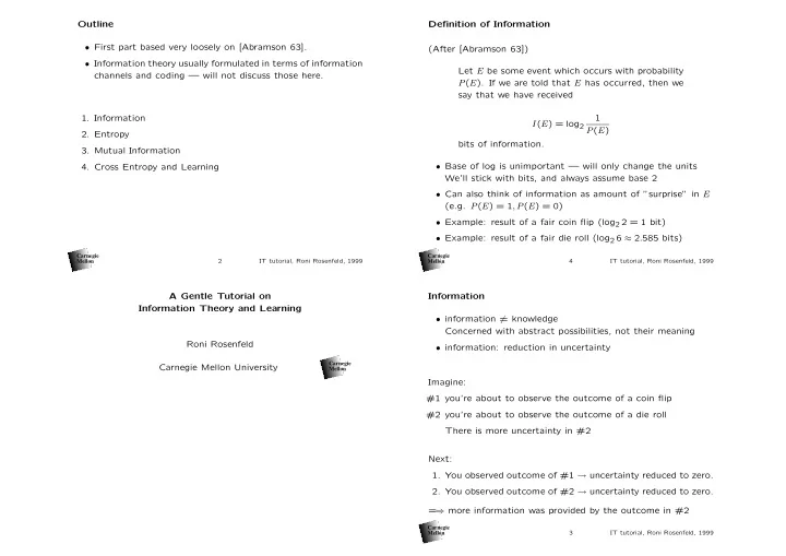
Outline Definition of Information First part based very loosely on - PowerPoint PPT Presentation

Outline Definition of Information • First part based very loosely on [Abramson 63]. (After [Abramson 63]) • Information theory usually formulated in terms of information Let E be some event which occurs with probability channels and coding — will not discuss those here. P ( E ). If we are told that E has occurred, then we say that we have received 1. Information 1 I ( E ) = log 2 P ( E ) 2. Entropy bits of information. 3. Mutual Information • Base of log is unimportant — will only change the units 4. Cross Entropy and Learning We’ll stick with bits, and always assume base 2 • Can also think of information as amount of ”surprise” in E (e.g. P ( E ) = 1 , P ( E ) = 0) • Example: result of a fair coin flip (log 2 2 = 1 bit) • Example: result of a fair die roll (log 2 6 ≈ 2 . 585 bits) Carnegie Carnegie Mellon Mellon 2 IT tutorial, Roni Rosenfeld, 1999 4 IT tutorial, Roni Rosenfeld, 1999 A Gentle Tutorial on Information Information Theory and Learning • information � = knowledge Concerned with abstract possibilities, not their meaning Roni Rosenfeld • information: reduction in uncertainty Carnegie Carnegie Mellon University Mellon Imagine: #1 you’re about to observe the outcome of a coin flip #2 you’re about to observe the outcome of a die roll There is more uncertainty in #2 Next: 1. You observed outcome of #1 → uncertainty reduced to zero. 2. You observed outcome of #2 → uncertainty reduced to zero. = ⇒ more information was provided by the outcome in #2 Carnegie Mellon 3 IT tutorial, Roni Rosenfeld, 1999

Entropy Entropy as a Function of a Probability Distribution A Zero-memory information source S is a source that emits sym- Since the source S is fully characterized by P = { p 1 , . . . p k } (we bols from an alphabet { s 1 , s 2 , . . . , s k } with probabilities { p 1 , p 2 , . . . , p k } , don’t care what the symbols s i actually are, or what they stand respectively, where the symbols emitted are statistically indepen- for), entropy can also be thought of as a property of a probability dent. distribution function P : the avg uncertainty in the distribution. So we may also write: What is the average amount of information in observing the output of the source S ? p i log 1 H ( S ) = H ( P ) = H ( p 1 , p 2 , . . . , p k ) = � p i Call this Entropy : i (Can be generalized to continuous distributions.) p i · log 1 1 � � H ( S ) = p i · I ( s i ) = = E P [ log p ( s ) ] p i i i * Carnegie Carnegie Mellon Mellon 6 IT tutorial, Roni Rosenfeld, 1999 8 IT tutorial, Roni Rosenfeld, 1999 Information is Additive Alternative Explanations of Entropy 1 • I ( k fair coin tosses) = log 1 / 2 k = k bits p i · log 1 • So: � H ( S ) = p i – random word from a 100,000 word vocabulary: i I(word) = log 100 , 000 = 16 . 61 bits 1. avg amt of info provided per symbol – A 1000 word document from same source: I(document) = 16,610 bits 2. avg amount of surprise when observing a symbol – A 480x640 pixel, 16-greyscale video picture: 3. uncertainty an observer has before seeing the symbol I(picture) = 307 , 200 · log 16 = 1 , 228 , 800 bits 4. avg # of bits needed to communicate each symbol • = ⇒ A (VGA) picture is worth (a lot more than) a 1000 words! (Shannon: there are codes that will communicate these sym- bols with efficiency arbitrarily close to H ( S ) bits/symbol; • (In reality, both are gross overestimates.) there are no codes that will do it with efficiency < H ( S ) bits/symbol) Carnegie Carnegie Mellon Mellon 5 IT tutorial, Roni Rosenfeld, 1999 7 IT tutorial, Roni Rosenfeld, 1999

Special Case: k = 2 The Entropy of English Flipping a coin with P(“head”)=p, P(“tail”)=1-p 27 characters (A-Z, space). 100,000 words (avg 5.5 characters each) H ( p ) = p · log 1 1 p + (1 − p ) · log • Assuming independence between successive characters: 1 − p – uniform character distribution: log 27 = 4 . 75 bits/character – true character distribution: 4.03 bits/character • Assuming independence between successive words : – unifrom word distribution: log 100 , 000 / 6 . 5 ≈ 2 . 55 bits/character – true word distribution: 9 . 45 / 6 . 5 ≈ 1 . 45 bits/character • True Entropy of English is much lower! Notice: • zero uncertainty/information/surprise at edges • maximum info at 0.5 (1 bit) • drops off quickly Carnegie Carnegie Mellon Mellon 10 IT tutorial, Roni Rosenfeld, 1999 12 IT tutorial, Roni Rosenfeld, 1999 Properties of Entropy Special Case: k = 2 (cont.) Relates to: ”20 questions” game strategy (halving the space). p i · log 1 � H ( P ) = p i So a sequence of (independent) 0’s-and-1’s can provide up to 1 i bit of information per digit, provided the 0’s and 1’s are equally 1. Non-negative: H ( P ) ≥ 0 likely at any point. If they are not equally likely, the sequence 2. Invariant wrt permutation of its inputs: provides less information and can be compressed . H ( p 1 , p 2 , . . . , p k ) = H ( p τ (1) , p τ (2) , . . . , p τ ( k ) ) 3. For any other probability distribution { q 1 , q 2 , . . . , q k } : p i · log 1 p i · log 1 � � H ( P ) = < p i q i i i 4. H ( P ) ≤ log k , with equality iff p i = 1 /k ∀ i 5. The further P is from uniform, the lower the entropy. Carnegie Carnegie Mellon Mellon 9 IT tutorial, Roni Rosenfeld, 1999 11 IT tutorial, Roni Rosenfeld, 1999

Joint Probability, Joint Entropy Conditional Probability, Conditional Entropy P ( M = m | T = t ) cold mild hot low 0.1 0.4 0.1 0.6 cold mild hot high 0.2 0.1 0.1 0.4 low 1/3 4/5 1/2 0.3 0.5 0.2 1.0 high 2/3 1/5 1/2 1.0 1.0 1.0 • H ( T ) = H (0 . 3 , 0 . 5 , 0 . 2) = 1 . 48548 Conditional Entropy: • H ( M ) = H (0 . 6 , 0 . 4) = 0 . 970951 • H ( M | T = cold ) = H (1 / 3 , 2 / 3) = 0 . 918296 • H ( T ) + H ( M ) = 2 . 456431 • H ( M | T = mild ) = H (4 / 5 , 1 / 5) = 0 . 721928 • Joint Entropy : consider the space of ( t, m ) events H ( T, M ) = • H ( M | T = hot ) = H (1 / 2 , 1 / 2) = 1 . 0 1 � t,m P ( T = t, M = m ) · log P ( T = t,M = m ) • Average Conditional Entropy (aka Equivocation): H (0 . 1 , 0 . 4 , 0 . 1 , 0 . 2 , 0 . 1 , 0 . 1) = 2 . 32193 H ( M/T ) = � t P ( T = t ) · H ( M | T = t ) = 0 . 3 · H ( M | T = cold ) + 0 . 5 · H ( M | T = mild ) + 0 . 2 · H ( M | T = hot ) = 0 . 8364528 Notice that H ( T, M ) < H ( T ) + H ( M ) !!! How much is T telling us on average about M ? H ( M ) − H ( M | T ) = 0 . 970951 − 0 . 8364528 ≈ 0 . 1345 bits Carnegie Carnegie Mellon Mellon 14 IT tutorial, Roni Rosenfeld, 1999 16 IT tutorial, Roni Rosenfeld, 1999 Two Sources Conditional Probability, Conditional Entropy P ( T = t | M = m ) Temperature T : a random variable taking on values t cold mild hot P(T=hot)=0.3 low 1/6 4/6 1/6 1.0 P(T=mild)=0.5 high 2/4 1/4 1/4 1.0 P(T=cold)=0.2 Conditional Entropy : = ⇒ H(T)=H(0.3, 0.5, 0.2) = 1.48548 • H ( T | M = low ) = H (1 / 6 , 4 / 6 , 1 / 6) = 1 . 25163 • H ( T | M = high ) = H (2 / 4 , 1 / 4 , 1 / 4) = 1 . 5 huMidity M : a random variable, taking on values m • Average Conditional Entropy (aka equivocation): P(M=low)=0.6 H ( T/M ) = � m P ( M = m ) · H ( T | M = m ) = P(M=high)=0.4 0 . 6 · H ( T | M = low ) + 0 . 4 · H ( T | M = high ) = 1 . 350978 = ⇒ H ( M ) = H (0 . 6 , 0 . 4) = 0 . 970951 How much is M telling us on average about T ? T, M not independent: P ( T = t, M = m ) � = P ( T = t ) · P ( M = m ) H ( T ) − H ( T | M ) = 1 . 48548 − 1 . 350978 ≈ 0 . 1345 bits Carnegie Carnegie Mellon Mellon 13 IT tutorial, Roni Rosenfeld, 1999 15 IT tutorial, Roni Rosenfeld, 1999

Mutual Information Visualized A Markov Source Order- k Markov Source: A source that ”remembers” the last k symbols emitted. Ie, the probability of emitting any symbol depends on the last k emitted symbols: P ( s T = t | s T = t − 1 , s T = t − 2 , . . . , s T = t − k ) So the last k emitted symbols define a state , and there are q k states. First-order markov source: defined by qXq matrix: P ( s i | s j ) Example: S T = t is position after t random steps H ( X, Y ) = H ( X ) + H ( Y ) − I ( X ; Y ) Carnegie Carnegie Mellon Mellon 18 IT tutorial, Roni Rosenfeld, 1999 20 IT tutorial, Roni Rosenfeld, 1999 Average Mutual Information Three Sources From Blachman: I ( X ; Y ) = H ( X ) − H ( X/Y ) 1 1 � � = P ( x ) · log P ( x ) − P ( x, y ) · log (”/” means ”given”. ”;” means ”between”. ”,” means ”and”.) P ( x | y ) x x,y P ( x, y ) · log P ( x | y ) = � • H ( X, Y/Z ) = H ( { X, Y } / Z ) P ( x ) x,y • H ( X/Y, Z ) = H ( X / { Y, Z } ) P ( x, y ) � = P ( x, y ) · log P ( x ) P ( y ) • I ( X ; Y/Z ) = H ( X/Z ) − H ( X/Y, Z ) x,y • Properties of Average Mutual Information: I ( X ; Y ; Z ) = I ( X ; Y ) − I ( X ; Y/Z ) = H ( X, Y, Z ) − H ( X, Y ) − H ( X, Z ) − H ( Y, Z ) + H ( X ) + H ( Y ) + H • Symmetric (but H ( X ) � = H ( Y ) and H ( X/Y ) � = H ( Y/X )) = ⇒ Can be negative! • Non-negative (but H ( X ) − H ( X/y ) may be negative!) • I ( X ; Y, Z ) = I ( X ; Y ) + I ( X ; Z/Y ) (additivity) • Zero iff X, Y independent • Additive (see next slide) • But: I ( X ; Y ) = 0, I ( X ; Z ) = 0 doesn’t mean I ( X ; Y, Z ) = 0!!! Carnegie Carnegie Mellon Mellon 17 IT tutorial, Roni Rosenfeld, 1999 19 IT tutorial, Roni Rosenfeld, 1999