Entropy Let X be a discrete random variable The surprise of - PDF document

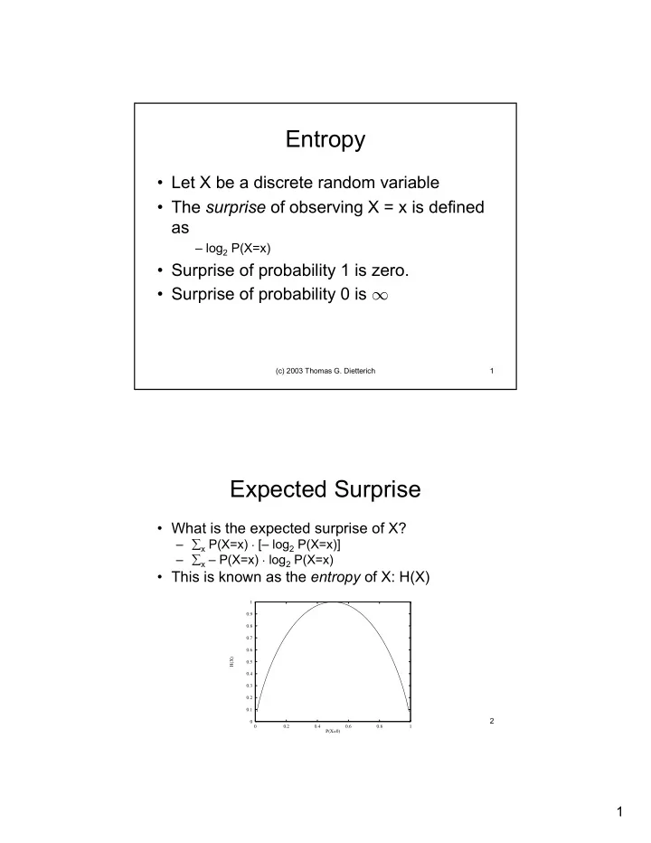
Entropy • Let X be a discrete random variable • The surprise of observing X = x is defined as – log 2 P(X=x) • Surprise of probability 1 is zero. • Surprise of probability 0 is ∞ (c) 2003 Thomas G. Dietterich 1 Expected Surprise • What is the expected surprise of X? – ∑ x P(X=x) · [– log 2 P(X=x)] – ∑ x – P(X=x) · log 2 P(X=x) • This is known as the entropy of X: H(X) 1 0.9 0.8 0.7 0.6 H(X) 0.5 0.4 0.3 0.2 0.1 (c) 2003 Thomas G. Dietterich 2 0 0 0.2 0.4 0.6 0.8 1 P(X=0) 1

Shannon’s Experiment • Measure the entropy of English – Ask humans to rank-order the next letter given all of the previous letters in a text. – Compute the position of the correct letter in this rank order – Produce a histogram – Estimate P(X| …) from this histogram – Compute the entropy H(X) = expected number of bits of “surprise” of seeing each new letter (c) 2003 Thomas G. Dietterich 3 Predicting the Next Letter Ever y t h i ng_in_camp_w as_drenched_the_camp_fire_as_well_for_they_ were but heedless lads like their generation and had made no provision against rain Here was matter for dismay for they were soaked through and chilled They were eloquent in their distress but they presently discovered that the fire had eaten so far up under the great log it had been built against where it curved upward and separated itself from the ground that a hand breadth or so of it had escaped wetting so they patiently wrought until with shreds and bark gathered from the under sides of sheltered logs they coaxed the fire to burn again Then they piled on great dead boughs till they had a roaring furnace and were glad hearted once more They dried their boiled ham and had a feast and after that they sat by the fire and expanded and glorified their midnight adventure until morning for there was not a dry spot to sleep on anywhere around (c) 2003 Thomas G. Dietterich 4 2

Statistical Learning Methods • The Density Estimation Problem: – Given: • a set of random variables U = {V 1 , …, V n } • A set S of training examples {U 1 , …, U N } drawn independently according to unknown distribution P(U) – Find: • A bayesian network with probabilities Θ that is a good approximation to P(U) • Four Cases: – Known Structure; Fully Observable – Known Structure; Partially Observable – Unknown Structure; Fully Observable – Unknown Structure; Partially Observable (c) 2003 Thomas G. Dietterich 5 Bayesian Learning Theory • Fundamental Question: Given S how to choose Θ ? • Bayesian Answer: Don’t choose a single Θ . (c) 2003 Thomas G. Dietterich 6 3

A Bayesian Network for Learning Bayesian Networks Θ … U U 1 U 2 U N P(U|U 1 ,…,U N ) = P(U|S) = P(U ∧ S) / P(S) = [ ∑ Θ P(U| Θ ) ∏ i P(U i | Θ ) · P( Θ )] / P(S) P(U|S) = ∑ Θ P(U| Θ ) · [P(S| Θ ) · P( Θ ) / P(S)] P(U|S) = ∑ Θ P(U| Θ ) · P( Θ | S) Each Θ votes for U according to its posterior probability. “Bayesian Model Averaging” (c) 2003 Thomas G. Dietterich 7 Approximating Bayesian Model Averaging • Summing over all possible Θ ’s is usually impossible. • Approximate this sum by the single most likely Θ value, Θ MAP • Θ MAP = argmax Θ P( Θ |S) = argmax Θ P(S| Θ ) P( Θ ) • P(U|S) ≈ P(U| Θ MAP ) • “Maximum Aposteriori Probability” – MAP (c) 2003 Thomas G. Dietterich 8 4

Maximum Likelihood Approximation • If we assume P( Θ ) is a constant for all Θ , then MAP become MLE, the Maximum Likelihood Estimate Θ MLE = argmax Θ P(S| Θ ) • P(S| Θ ) is called the “likelihood function” • We often take logarithms Θ MLE = argmax Θ P(S| Θ ) = argmax Θ log P(S| Θ ) = argmax Θ log ∏ i P(U i | Θ ) = argmax Θ ∑ i log P(U i | Θ ) (c) 2003 Thomas G. Dietterich 9 Experimental Methodology • Collect data • Divide data randomly into training and testing sets • Choose Θ to maximize log likelihood of the training data • Evaluate log likelihood on the test data (c) 2003 Thomas G. Dietterich 10 5

Known Structure, Fully Observable Age Preg Preg Glucose Insulin Mass Age Diabetes? 3 3 1 2 3 0 3 2 3 3 6 0 Mass 3 4 0 3 3 0 3 1 1 3 4 0 3 5 0 3 4 1 Diabetes 1 1 0 3 4 1 2 0 3 3 2 0 2 8 2 4 2 1 Insulin 1 2 0 3 4 0 3 2 1 3 4 0 Glucose (c) 2003 Thomas G. Dietterich 11 Learning Process • Simply count the cases: P ( Age = 2) = N ( Age = 2) N P ( Mass = 0 | Preg = 1 , Age = 2) = N ( Mass = 0 , Preg = 1 , Age = 2) N ( Preg = 1 , Age = 2) (c) 2003 Thomas G. Dietterich 12 6

Laplace Corrections • Probabilities of 0 and 1 are undesirable because they are too strong. To avoid them, we can apply the Laplace Correction. Suppose there are k possible values for age: P ( Age = 2) = N ( Age = 2) + 1 N + k • Implementation: Initialize all counts to 1. When the counts are normalized, this automatically computes k . (c) 2003 Thomas G. Dietterich 13 Spam Filtering using Naïve Bayes Spam … money confidential nigeria machine learning • Spam ∈ {0,1} • One random variable for each possible word that could appear in email • P(money=1 | Spam=1); P(money=1 | Spam=0) (c) 2003 Thomas G. Dietterich 14 7

Probabilistic Reasoning • All of the variables are observed except Spam, so the reasoning is very simple: P(spam=1|w 1 ,w 2 ,…,w n ) = α P(w 1 |spam=1) · P(w 2 |spam=1) · · · P(w n |spam=1) · P(spam=1) (c) 2003 Thomas G. Dietterich 15 Likelihood Ratio • To avoid normalization, we can compute the “log odds”: P ( spam = 0 | w = 1 , . . . , w n ) = α P ( w 1 | spam = 1) · · · P ( w n | spam = 1) · P ( spam = 1) P ( spam = 1 | w 1 , . . . , w n ) α P ( w 1 | spam = 0) · · · P ( w n | spam = 0) · P ( spam = 0) P ( spam = 1 | w 1 , . . . , w n ) α · P ( w 1 | spam = 1) P ( w 1 | spam = 0) · · · P ( w n | spam = 1) P ( w n | spam = 0) · P ( spam = 1) P ( spam = 0 | w = 1 , . . . , w n ) = α P ( spam = 0) P ( spam = 0 | w = 1 , . . . , w n ) = log P ( w 1 | spam = 1) P ( spam = 1 | w 1 , . . . , w n ) P ( w 1 | spam = 0)+ . . . +log P ( w n | spam = 1) P ( w n | spam = 0)+log P ( spam = 1) log P ( spam = 0) (c) 2003 Thomas G. Dietterich 16 8

Design Issues • What to consider “words”? – Read Paul Graham’s articles (see web page) – Read about CRM114 – Do we define w j to be the number of times w j appears in the email? Or do we just use a boolean: presence/absence of the word? • How to handle previously unseen words? – Laplace estimates will assign them probabilities of 0.5 and 0.5 and NB will therefore ignore them. • Efficient implementation – Two hash tables: one for spam and one for non-spam that contain the counts of the number of messages in which the word was seen. (c) 2003 Thomas G. Dietterich 17 Correlations? • Naïve Bayes assumes that each word is generated independently given the class. • HTML tokens are not generated independently. Should we model this? Spam HTML … money confidential nigeria <b> href (c) 2003 Thomas G. Dietterich 18 9

Dynamics • We are engaged in an “arms race” between the spammers and the spam filters. Spam is changing all the time, so we need our estimates P(w i |spam) to be changing too. • One Method: Exponential moving average. Each time we process a new training message, we decay the previous counts slightly. For every w i : – N(w i |spam=1) := N(w i |spam=1) · 0.9999 – N(w i |spam=0) := N(w i |spam=0) · 0.9999 Then add in the counts for the new words. Choose the constant (0.9999) carefully. (c) 2003 Thomas G. Dietterich 19 Decay Parameter 1 0.9999**x 0.9 0.8 0.7 0.6 0.5 0.4 0.3 0.2 0.1 0 0 5000 10000 15000 20000 25000 30000 35000 40000 45000 50000 • “half life” is 6930 updates (how did I compute that?) (c) 2003 Thomas G. Dietterich 20 10

Architecture • .procmailrc is read by sendmail on engr accounts. This allows you to pipe your email into a program you write yourself. # .procmail recipe # pipe mail into myprogram, then continue processing it :0fw: .msgid.lock | /home/tgd/myprogram # if myprogram added the spam header, then file into # the spam mail file :0: * ^X-SPAM-Status: SPAM.* mail/spam (c) 2003 Thomas G. Dietterich 21 Architecture (2) • Tokenize • Hash • Classify (c) 2003 Thomas G. Dietterich 22 11

Classification Decision • False positives: good email misclassified as spam • False negatives: spam misclassified as good email • Choose a threshold θ P ( spam = 1 | w 1 , . . . , w n ) log P ( spam = 0 | w = 1 , . . . , w n ) > θ (c) 2003 Thomas G. Dietterich 23 Plot of False Positives versus False Negatives As we vary θ , we 800 30 change the 700 29 number of false 28 600 27 26 25 positives and false 24 500 23 False Negatives 22 negatives. We 21 20 400 19 can choose the 18 17 16 300 15 1 threshold that 14 2 13 4 3 12 11 5 7 6 10 9 8 200 achieves the -10*FP -1*FP 100 desired ratio of FP to FN 0 0 50 100 150 200 250 300 350 400 False Positives (c) 2003 Thomas G. Dietterich 24 12