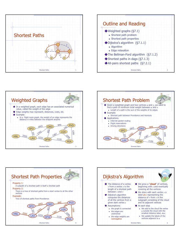
Outline and Reading Weighted graphs (7.1) Shortest Paths Shortest - - PDF document

SLIDE 1

Shortest Paths 1

Shortest Paths

C B A E D F 3 2 8 5 8 4 8 7 1 2 5 2 3 9

Shortest Paths 2

Outline and Reading

Weighted graphs (§7.1)

Shortest path problem Shortest path properties

Dijkstra’s algorithm (§7.1.1)

Algorithm Edge relaxation

The Bellman-Ford algorithm (§7.1.2) Shortest paths in dags (§7.1.3) All-pairs shortest paths (§7.2.1)

Shortest Paths 3

Weighted Graphs

In a weighted graph, each edge has an associated numerical value, called the weight of the edge Edge weights may represent, distances, costs, etc. Example:

In a flight route graph, the weight of an edge represents the

distance in miles between the endpoint airports

ORD PVD MIA DFW SFO LAX LGA HNL

8 4 9 802 1387 1743 1 8 4 3 1099 1120 1233 337 2555 142 1205

Shortest Paths 4

Shortest Path Problem

Given a weighted graph and two vertices u and v, we want to find a path of minimum total weight between u and v.

Length of a path is the sum of the weights of its edges.

Example:

Shortest path between Providence and Honolulu

Applications

Internet packet routing Flight reservations Driving directions

ORD PVD MIA DFW SFO LAX LGA HNL

8 4 9 802 1387 1743 1 8 4 3 1099 1120 1233 337 2555 142 1205

Shortest Paths 5

Shortest Path Properties

Property 1:

A subpath of a shortest path is itself a shortest path

Property 2:

There is a tree of shortest paths from a start vertex to all the other vertices

Example:

Tree of shortest paths from Providence

ORD PVD MIA DFW SFO LAX LGA HNL

8 4 9 802 1387 1743 1 8 4 3 1099 1120 1233 337 2555 142 1205

Shortest Paths 6

Dijkstra’s Algorithm

The distance of a vertex v from a vertex s is the length of a shortest path between s and v Dijkstra’s algorithm computes the distances

• f all the vertices from a

given start vertex s Assumptions:

the graph is connected the edges are

undirected

the edge weights are

nonnegative

We grow a “cloud” of vertices, beginning with s and eventually covering all the vertices We store with each vertex v a label d(v) representing the distance of v from s in the subgraph consisting of the cloud and its adjacent vertices At each step

We add to the cloud the vertex

u outside the cloud with the smallest distance label, d(u)

We update the labels of the

vertices adjacent to u

SLIDE 2

Shortest Paths 7

Edge Relaxation

Consider an edge e = (u,z) such that

u is the vertex most recently

added to the cloud

z is not in the cloud

The relaxation of edge e updates distance d(z) as follows:

d(z) ← min{d(z),d(u) + weight(e)}

d(z) = 75

d(u) = 50 10 z s u

d(z) = 60

d(u) = 50 10 z s u e e

Shortest Paths 8

Example

C B A E D F 4 2 8 ∞ ∞ 4 8 7 1 2 5 2 3 9 C B A E D F 3 2 8 5 11 4 8 7 1 2 5 2 3 9 C B A E D F 3 2 8 5 8 4 8 7 1 2 5 2 3 9 C B A E D F 3 2 7 5 8 4 8 7 1 2 5 2 3 9

Shortest Paths 9

Example (cont.)

C B A E D F 3 2 7 5 8 4 8 7 1 2 5 2 3 9 C B A E D F 3 2 7 5 8 4 8 7 1 2 5 2 3 9

Shortest Paths 10

Dijkstra’s Algorithm

A priority queue stores the vertices outside the cloud

Key: distance Element: vertex

Locator-based methods

insert(k,e) returns a

locator

replaceKey(l,k) changes

the key of an item

We store two labels with each vertex:

Distance (d(v) label) locator in priority

queue Algorithm DijkstraDistances(G, s) Q ← new heap-based priority queue for all v ∈ G.vertices() if v = s setDistance(v, 0) else setDistance(v, ∞) l ← Q.insert(getDistance(v), v) setLocator(v,l) while ¬Q.isEmpty() u ← Q.removeMin() for all e ∈ G.incidentEdges(u) { relax edge e } z ← G.opposite(u,e) r ← getDistance(u) + weight(e) if r < getDistance(z) setDistance(z,r) Q.replaceKey(getLocator(z),r)

Shortest Paths 11

Analysis

Graph operations

Method incidentEdges is called once for each vertex

Label operations

We set/get the distance and locator labels of vertex z O(deg(z)) times Setting/getting a label takes O(1) time

Priority queue operations

Each vertex is inserted once into and removed once from the priority

queue, where each insertion or removal takes O(log n) time

The key of a vertex in the priority queue is modified at most deg(w)

times, where each key change takes O(log n) time

Dijkstra’s algorithm runs in O((n + m) log n) time provided the graph is represented by the adjacency list structure

Recall that Σv deg(v) = 2m

The running time can also be expressed as O(m log n) since the graph is connected

Shortest Paths 12

Extension

Using the template method pattern, we can extend Dijkstra’s algorithm to return a tree of shortest paths from the start vertex to all other vertices We store with each vertex a third label:

parent edge in the

shortest path tree

In the edge relaxation step, we update the parent label

Algorithm DijkstraShortestPathsTree(G, s) … for all v ∈ G.vertices() … setParent(v, ∅) … for all e ∈ G.incidentEdges(u) { relax edge e } z ← G.opposite(u,e) r ← getDistance(u) + weight(e) if r < getDistance(z) setDistance(z,r) setParent(z,e) Q.replaceKey(getLocator(z),r)

SLIDE 3

Shortest Paths 13

Why Dijkstra’s Algorithm Works

Dijkstra’s algorithm is based on the greedy

• method. It adds vertices by increasing distance.

C B A E D F 3 2 7 5 8 4 8 7 1 2 5 2 3 9

Suppose it didn’t find all shortest

• distances. Let F be the first wrong

vertex the algorithm processed.

When the previous node, D, on the

true shortest path was considered, its distance was correct.

But the edge (D,F) was relaxed at

that time!

Thus, so long as d(F)>d(D), F’s

distance cannot be wrong. That is, there is no wrong vertex.

Shortest Paths 14

Why It Doesn’t Work for Negative-Weight Edges

If a node with a negative

incident edge were to be added late to the cloud, it could mess up distances for vertices already in the cloud.

C B A E D F 4 5 7 5 9 4 8 7 1 2 5 6

• 8

Dijkstra’s algorithm is based on the greedy

• method. It adds vertices by increasing distance.

C’s true distance is 1, but it is already in the cloud with d(C)=5!

Shortest Paths 15

Bellman-Ford Algorithm

Works even with negative- weight edges Must assume directed edges (for otherwise we would have negative- weight cycles) Iteration i finds all shortest paths that use i edges. Running time: O(nm). Can be extended to detect a negative-weight cycle if it exists

How?

Algorithm BellmanFord(G, s) for all v ∈ G.vertices() if v = s setDistance(v, 0) else setDistance(v, ∞) for i ← 1 to n-1 do for each e ∈ G.edges() { relax edge e } u ← G.origin(e) z ← G.opposite(u,e) r ← getDistance(u) + weight(e) if r < getDistance(z) setDistance(z,r)

Shortest Paths 16

∞

• 2

Bellman-Ford Example

∞ ∞ ∞ ∞ ∞ 4 8 7 1

• 2

5

• 2

3 9 ∞ ∞ ∞ ∞ 4 8 7 1

• 2

5 3 9

Nodes are labeled with their d(v) values

• 2
• 2

8 4 ∞ 4 8 7 1

• 2

5 3 9 ∞ 8

• 2

4

• 1

5 6 1 9

• 2

5 1

• 1

9 4 8 7 1

• 2

5

• 2

3 9 4

Shortest Paths 17

DAG-based Algorithm

Works even with negative-weight edges Uses topological order Doesn’t use any fancy data structures Is much faster than Dijkstra’s algorithm Running time: O(n+m).

Algorithm DagDistances(G, s) for all v ∈ G.vertices() if v = s setDistance(v, 0) else setDistance(v, ∞) Perform a topological sort of the vertices for u ← 1 to n do {in topological order} for each e ∈ G.outEdges(u) { relax edge e } z ← G.opposite(u,e) r ← getDistance(u) + weight(e) if r < getDistance(z) setDistance(z,r)

Shortest Paths 18

∞

• 2

DAG Example

∞ ∞ ∞ ∞ ∞ 4 8 7 1

• 5

5

• 2

3 9 ∞ ∞ ∞ ∞ 4 8 7 1

• 5

5 3 9

Nodes are labeled with their d(v) values

• 2
• 2

8 4 ∞ 4 8 7 1

• 5

5 3 9 ∞

• 2

4

• 1

1 7

• 2

5 1

• 1

7 4 8 7 1

• 5

5

• 2

3 9 4

1 1 2 4 3 6 5 1 2 4 3 6 5

8

1 2 4 3 6 5 1 2 4 3 6 5

5

(two steps)

SLIDE 4

Shortest Paths 19

All-Pairs Shortest Paths

Find the distance between every pair of vertices in a weighted directed graph G. We can make n calls to Dijkstra’s algorithm (if no negative edges), which takes O(nmlog n) time. Likewise, n calls to Bellman-Ford would take O(n2m) time. We can achieve O(n3) time using dynamic programming (similar to the Floyd-Warshall algorithm).

Algorithm AllPair(G) {assumes vertices 1,…,n} for all vertex pairs (i,j) if i = j D0[i,i] ← 0 else if (i,j) is an edge in G D0[i,j] ← weight of edge (i,j) else D0[i,j] ← + ∞ for k ← 1 to n do for i ← 1 to n do for j ← 1 to n do Dk[i,j] ← min{Dk-1[i,j], Dk-1[i,k]+Dk-1[k,j]} return Dn

k j i

Uses only vertices numbered 1,…,k-1 Uses only vertices numbered 1,…,k-1 Uses only vertices numbered 1,…,k (compute weight of this edge)