[PDF] - Out line Decision Net works Aka I nf luence diagr ams Lect ure PDF Document

SLIDE 1

1 Lect ure 11

J une 7, 2005 CS 486/ 686

2

Out line

Decision Net works

– Aka I nf luence diagr ams

Value of inf ormat ion
Russell and Norvig: Sect 16.5-16.6

3

Decision Net works

Decision net wor ks (also known as

inf luence diagr ams) provide a way of represent ing sequent ial decision problems

– basic idea: represent t he variables in t he problem as you would in a BN – add decision variables – variables t hat you “cont r ol” – add ut ilit y variables – how good dif f erent st at es are

4

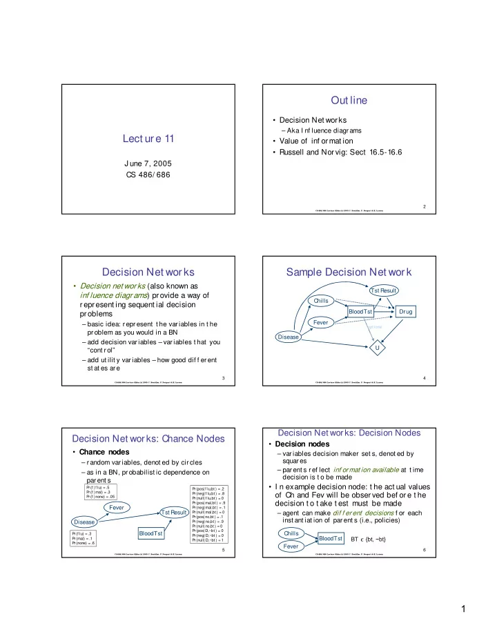
Sample Decision Net work

Disease Tst Result Chills Fever BloodTst Drug U

pt ional

5

Decision Net wor ks: Chance Nodes

Chance nodes

– random var iables, denot ed by circles – as in a BN, probabilist ic dependence on parent s

Disease Fever

Pr(f lu) = .3 Pr(mal) = .1 Pr(none) = .6 Pr(f | f lu) = .5 Pr(f | mal) = .3 Pr(f | none) = .05

Tst Result BloodTst

6

Decision Net works: Decision Nodes

Decision nodes

– variables decision maker set s, denot ed by squares – parent s ref lect inf ormat ion available at t ime decision is t o be made

I n example decision node: t he act ual values
f Ch and Fev will be observed bef ore t he

decision t o t ake t est must be made

– agent can make dif f erent decisions f or each inst ant iat ion of parent s (i.e., policies)

Chills Fever BloodTst BT ∊ {bt, ~bt}

SLIDE 2

2

7

Decision Net wor ks: Value Node

Value node

– specif ies ut ilit y of a st at e, denot ed by a diamond – ut ilit y depends only on st at e of parent s of value node – generally: only one value node in a decision net work

Ut ilit y depends only on disease and drug

Disease BloodTst Drug U

pt ional

U(f ludrug, f lu) = 20 U(f ludrug, mal) = -300 U(f ludrug, none) = -5 U(maldrug, f lu) = -30 U(maldrug, mal) = 10 U(maldrug, none) = -20 U(no drug, f lu) = -10 U(no drug, mal) = -285 U(no drug, none) = 30

8

Decision Net wor ks: Assumpt ions

Decision nodes are t ot ally ordered

– decision variables D1, D2, … , Dn – decisions are made in sequence – e.g., BloodTst (yes,no) decided bef ore Drug (f d,md,no)

No-f orget t ing propert y

– any inf ormat ion available when decision Di is made is available when decision Dj is made (f or i < j ) – t hus all parent s of Di are parent s of Dj Chills Fever BloodTst Drug

Dashed ar cs ensure t he no-f orget t ing pr oper t y

9

Policies

Let Par(Di) be t he parent s of decision node Di

– Dom(Par(Di)) is t he set of assignment s t o parent s

A policy δ is a set of mappings δi, one f or each

decision node Di

– δi :Dom(Par(Di)) →Dom(Di) – δi associat es a decision wit h each parent asst f or Di

For example, a policy f or BT might be:

– δBT (c,f ) = bt – δBT (c,~f ) = ~bt – δBT (~c,f ) = bt – δBT (~c,~f ) = ~bt Chills Fever BloodTst

10

Value of a Policy

Value of a policy δ is t he expect ed ut ilit y given

t hat decision nodes are execut ed according t o δ

Given asst x t o t he set X of all chance

variables, let δ(x) denot e t he asst t o decision variables dict at ed by δ

– e.g., asst t o D1 det ermined by it ’s parent s’ asst in x – e.g., asst t o D2 det ermined by it ’s parent s’ asst in x along wit h what ever was assigned t o D1 – etc.

Value of δ :

EU(δ) = ΣX P(X, δ(X)) U(X, δ(X))

11

Opt imal Policies

An opt imal policy is a policy δ* such t hat

EU(δ*) ≥ EU(δ) f or all policies δ

We can use t he dynamic pr ogramming

principle yet again t o avoid enumerat ing all policies

We can also use t he st ruct ure of t he

decision net work t o use var iable eliminat ion t o aid in t he comput at ion

12

Comput ing t he Best Policy

We can work backwards as f ollows
First comput e opt imal policy f or Drug (last

dec’n)

– f or each asst t o parent s (C,F,BT,TR) and f or each decision value (D = md,f d,none), comput e t he expect ed value of choosing t hat value of D – set policy choice f or each value of parent s t o be t he value of D t hat has max value – eg: δD(c,f ,bt ,pos) = md

Disease Tst Result Chills Fever BloodTst Drug U

pt ional

SLIDE 3

3

13

Comput ing t he Best Policy

Next comput e policy f or BT given policy

δD(C,F,BT,TR) j ust det er mined f or Drug

– since δD(C,F,BT,TR) is f ixed, we can t reat Drug as a normal r andom var iable wit h det erminist ic pr obabilit ies – i.e., f or any inst ant iat ion of par ent s, value

f Drug is f ixed by policy δD

– t his means we can solve f or opt imal policy f or BT j ust as bef ore – only uninst ant iat ed vars are r andom vars (once we f ix it s parent s)

14

Comput ing t he Best Policy

How do we comput e t hese expect ed values?

– suppose we have asst < c,f ,bt ,pos>t o parent s of Drug – we want t o comput e EU of deciding t o set Drug = md – we can run variable eliminat ion!

Treat C,F,BT,TR,Dr as evidence

– t his reduces f act ors (e.g., U rest rict ed t o bt ,md: depends on Dis) – eliminat e remaining variables (e.g., only Disease lef t ) – lef t wit h f act or: EU(md| c, f , bt, pos) =

ΣDis P(Dis| c, f , bt, pos, md) U(Dis, bt, md)

We now know EU of doing

Dr=md when c,f ,bt ,pos t rue

Can do same f or f d,no t o

decide which is best

Disease Tst Result Chills Fever BloodTst Drug U

pt ional

15

Comput ing Expect ed Ut ilit ies

The preceding illust r at es a gener al

phenomenon

– comput ing expect ed ut ilit ies wit h BNs is quit e easy – ut ilit y nodes are j ust f act ors t hat can be dealt wit h using variable eliminat ion EU = ΣA,B,C P(A,B,C) U(B,C) = ΣA,B,C P(C| B) P(B| A) P(A) U(B,C)

J ust eliminat e variables

in t he usual way

U C B A

16

Opt imizing Policies: Key Point s

I f a decision node D has no decisions t hat

f ollow it , we can f ind it s policy by inst ant iat ing each of it s parent s and comput ing t he expect ed ut ilit y of each decision f or each parent inst ant iat ion

– no-f orget t ing means t hat all ot her decisions are inst ant iat ed (t hey must be parent s) – it s easy t o comput e t he expect ed ut ilit y using VE – t he number of comput at ions is quit e large: we run expect ed ut ilit y calculat ions (VE) f or each parent inst ant iat ion t oget her wit h each possible decision D might allow – policy: choose max decision f or each parent inst ant ’n

17

Opt imizing Policies: Key Point s

When a decision D node is opt imized, it can be

t reat ed as a random variable

– f or each inst ant iat ion of it s parent s we now know what value t he decision should t ake – j ust t reat policy as a new CPT: f or a given parent inst ant iat ion x, D get s δ(x) wit h probabilit y 1(all

t her decisions get probabilit y zero)
I f we opt imize f rom last decision t o f irst , at

each point we can opt imize a specif ic decision by (a bunch of ) simple VE calculat ions

– it ’s successor decisions (opt imized) are j ust normal nodes in t he BNs (wit h CPTs)

18

Decision Net work Not es

Decision net works commonly used by decision

analyst s t o help st ruct ure decision problems

Much work put int o comput at ionally ef f ect ive

t echniques t o solve t hese

– common t rick: replace t he decision nodes wit h random variables at out set and solve a plain Bayes net (a subt le but usef ul t ransf ormat ion)

Complexit y much great er t han BN inf erence

– we need t o solve a number of BN inf erence problems – one BN problem f or each set t ing of decision node parent s and decision node value

SLIDE 4

4

19

A Decision Net Example

Set t ing: you want t o buy a used car, but t here’s

a good chance it is a “lemon” (i.e., prone t o breakdown). Bef ore deciding t o buy it , you can t ake it t o a mechanic f or inspect ion. S/ he will give you a report on t he car, labelling it eit her “good” or “bad”. A good report is posit ively cor relat ed wit h t he car being sound, while a bad report is posit ively cor relat ed wit h t he car being a lemon.

The report cost s $50 however. So you could

risk it , and buy t he car wit hout t he report .

Owning a sound car is bet t er t han having no car ,

which is bet t er t han owning a lemon.

20

Car Buyer’s Net work

Lemon Report I nspect Buy U l ~l 0.5 0.5 g b n l i 0.2 0.8 0 ~l i 0.9 0.1 0 l ~i 0 0 1 ~l ~i 0 0 1 Rep: good,bad,none b l -600 b ~l 1000 ~b l -300 ~b~l

300

Ut ilit y

50 if

inspect

21

Evaluat e Last Decision: Buy (1)

EU(B| I ,R) = ΣL P(L| I ,R,B) U(L,I ,B)
I = i, R = g:

– EU(buy) = P(l| i,g,buy) U(l,i,buy) + P(~l| i,g,buy) U(~l,i,buy)

= .18*-650 + .82*950 = 662

– EU(~buy) = P(l| i,g,~buy) U(l,i,~buy) + P(~l| i,g,~buy) U(~l,i,~buy)

= -300 - 50 = -350 (-300 indep. of lemon)

– So opt imal δBuy (i,g) = buy

22

Evaluat e Last Decision: Buy (2)

I = i, R = b:

– EU(buy) = P(l| i,b,buy) U(l,i,buy) + P(~l| i,b,buy) U(~l,i,buy)

= .89*-650 + .11*950 = -474

– EU(~buy) = P(l| i,b,~buy) U(l,i,~buy) + P(~l| i, b,~buy) U(~l,i,~buy)

= -300 - 50 = -350 (-300 indep. of lemon)

– So opt imal δBuy (i,b) = ~buy

23

Evaluat e Last Decision: Buy (3)

I = ~i, R = n

– EU(buy) = P(l|~i,n,buy) U(l,~i,buy) + P(~l|~i,n,buy) U(~l,~i,buy)

= .5*-600 + .5*1000 = 200

– EU(~buy) = P(l|~i,n,~buy) U(l,~i,~buy) + P(~l| ~i,n,~buy) U(~l,~i,~buy)

= -300 (-300 indep. of lemon)

– So opt imal δBuy (~i,n) = buy

So opt imal policy f or Buy is:

– δBuy (i,g) = buy ; δBuy (i,b) = ~buy ; δBuy (~i,n) = buy

Not e: we don’t bot her comput ing policy f or

(i,~n), (~i, g), or (~i, b), since t hese occur wit h probabilit y 0

24

Using Variable Eliminat ion

Rest rict ion: replace f 2(L,I ,R) by f 4(L) = f 2(L,i,g) replace f 3(L,I ,B) by f 5(L,B) = f 2(L,i,B) St ep 1: Add f 6(B)= ΣL f 1(L) f 4(L) f 5(L,B) Remove: f 1(L), f 4(L), f 5(L,B) Last f act or: f 6(B) is t he unscaled expect ed ut ilit y of buy and ~buy. Select act ion wit h highest (unscaled) expect ed ut ilit y. Repeat f or EU(B|i,b), EU(B|~i,n) Factors: f 1(L) f 2(L,I ,R) f 3(L,I ,B) Query: EU(B)? Evidence: I = i, R = g

Elim. Order: L

L

f 1(L) f 3(L,I ,B) f 2(L,I ,R)

R

I B

U

SLIDE 5

5

25

Alt ernat ively

N.B.: variable eliminat ion f or decision net works

comput es unscaled expect ed ut ilit y…

Can st ill pick best act ion, since ut ilit y scale is

not import ant (relat ive magnit ude is what mat t ers)

I f we want exact expect ed ut ilit y:

– Let X = parent s(U) – EU(dec| evidence) = ΣX Pr(X|dec,evidence) U(X) – Comput e Pr(X|dec,evidence) by variable eliminat ion – Mult iply Pr(X|dec,evidence) by U(X) – Summout X

26

Evaluat e Fir st Decision: I nspect

EU(I ) = ΣL,R P(L,R| i) U(L,i,δBuy (I , R))

– where P(R,L|i) = P(R|L,i)P(L|i) – EU(i) = (.1)(-650)+(.4)(-350)+(.45)(950)+(.05)(-350)

= 187.5

– EU(~i) = P(n,l| ~i) U(l,~i,buy) + P(n,~l| ~i) U(~l,~i,buy)

= .5*-600 + .5*1000 = 200

– So opt imal δI nspect () = ~inspect

300 - 50 = -350

~buy 0.05 b,~l 1000 - 50 = 950 buy 0.45 g,~l

300 - 50 = -350

~buy 0.4 b,l

600 - 50 = -650

buy 0.1 g,l U( L, i, δBuy ) δBuy P(R,L | i)

27

Using Variable Eliminat ion

N.B. f 3(R,I ,B) = δB(R,I ) St ep 1: Add f 5(R,I ,B)= ΣL f 1(L) f 2(L,I ,R) f 4(L,I ,B) Remove: f 1(L) f 2(L,I ,R) f 4(L,I ,B) St ep 2: Add f 6(I ,B)= ΣR f 3(R,I ,B) f 5(R,I ,B) Remove: f 3(R,I ,B) f 5(R,I ,B) St ep 3: Add f 7(I )= ΣB f 6(I ,B) Remove: f 6(I ,B) Last f act or: f 7(I ) is t he expect ed ut ilit y of inspect and ~inspect . Select act ion wit h highest expect ed ut ilit y. Fact ors: f 1(L) f 2(L,I ,R) f 3(R,I ,B) f 4(L,I ,B) Query: EU(I )? Evidence: none

Elim. Order: L, R, B

L

f 1(L) f 4(L,I ,B) f 2(L,I ,R)

R

I B

U

f 3(R,I ,B)

28

Value of I nf ormat ion

So opt imal policy is: don’t inspect , buy t he car

– EU = 200 – Not ice t hat t he EU of inspect ing t he car, t hen buying it if f you get a good report , is 237.5 less t he cost of t he inspect ion (50). So inspect ion not wort h t he improvement in EU. – But suppose inspect ion cost $25: t hen it would be wort h it (EU = 237.5 – 25 = 212.5 > EU(~i)) – The expect ed value of inf ormat ion associat ed wit h inspect ion is 37.5 (it improves expect ed ut ilit y by t his amount ignoring cost of inspect ion). How? Gives

pport unit y t o change decision (~buy if bad).

– You should be willing t o pay up t o $37.5 f or t he report

29

Next Class

Reasoning under uncer t aint y over t ime

– I nf erence in t emporal models – Hidden Markov Models – Dynamic Bayesian Net works

Russell and Norvig: Chapt er 15