Our Status in CS188 CS 188: Artificial Intelligence We re done - PDF document

Our Status in CS188 CS 188: Artificial Intelligence § We ’ re done with Part I Search and Planning! § Part II: Probabilistic Reasoning § Diagnosis Probability § Tracking objects § Speech recognition § Robot mapping § Genetics § Error correcting codes § … lots more! Pieter Abbeel – UC Berkeley Many slides adapted from Dan Klein. § Part III: Machine Learning 1 2 Part II: Probabilistic Reasoning Probability § Probability § Probability § Random Variables § Distributions over LARGE Numbers of § Joint and Marginal Distributions Random Variables § Conditional Distribution § Inference by Enumeration § Representation § Product Rule, Chain Rule, Bayes ’ Rule § Independence § Independence § You ’ ll need all this stuff A LOT for the next few weeks, § Inference so make sure you go over it now and know it inside out! § Variable Elimination The next few weeks we will learn how to make these § Sampling work computationally efficiently for LARGE numbers of § Hidden Markov Models random variables. 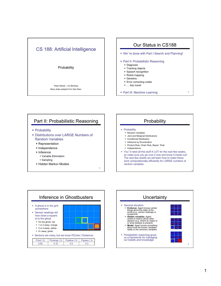3 4 Inference in Ghostbusters Uncertainty § General situation: § A ghost is in the grid § Evidence : Agent knows certain somewhere things about the state of the § Sensor readings tell world (e.g., sensor readings or symptoms) how close a square § Hidden variables : Agent is to the ghost needs to reason about other aspects (e.g. where an object is § On the ghost: red or what disease is present) § 1 or 2 away: orange § Model : Agent knows something about how the known variables § 3 or 4 away: yellow relate to the unknown variables § 5+ away: green § Probabilistic reasoning gives § Sensors are noisy, but we know P(Color | Distance) us a framework for managing our beliefs and knowledge P(red | 3) P(orange | 3) P(yellow | 3) P(green | 3) 0.05 0.15 0.5 0.3 6 1

Random Variables Probability Distributions § Unobserved random variables have distributions § A random variable is some aspect of the world about which we (may) have uncertainty § R = Is it raining? T P W P § D = How long will it take to drive to work? warm 0.5 sun 0.6 § L = Where am I? cold 0.5 rain 0.1 fog 0.3 § We denote random variables with capital letters meteor 0.0 § A distribution is a TABLE of probabilities of values § Like variables in a CSP, random variables have domains § A probability (lower case value) is a single number § R in {true, false} (sometimes write as {+r, ¬ r}) § D in [0, ∞ ) § L in possible locations, maybe {(0,0), (0,1), … } § Must have: 7 8 Joint Distributions Probabilistic Models Distribution over T,W § A probabilistic model is a joint distribution § A joint distribution over a set of random variables: over a set of random variables specifies a real number for each assignment (or outcome ): T W P hot sun 0.4 § Probabilistic models: § (Random) variables with domains hot rain 0.1 Assignments are called outcomes T W P cold sun 0.2 § Joint distributions: say whether hot sun 0.4 assignments (outcomes) are likely § Size of distribution if n variables with domain sizes d? cold rain 0.3 § Normalized: sum to 1.0 hot rain 0.1 § Ideally: only certain variables directly § Must obey: cold sun 0.2 Constraint over T,W interact cold rain 0.3 T W P § Constraint satisfaction probs: hot sun T § Variables with domains § Constraints: state whether assignments hot rain F are possible cold sun F § Ideally: only certain variables directly § For all but the smallest distributions, impractical to write out interact cold rain T 9 10 Events Marginal Distributions § Marginal distributions are sub-tables which eliminate variables § An event is a set E of outcomes T W P § Marginalization (summing out): Combine collapsed rows by adding hot sun 0.4 hot rain 0.1 T P cold sun 0.2 § From a joint distribution, we can calculate hot 0.5 cold rain 0.3 the probability of any event T W P cold 0.5 hot sun 0.4 § Probability that it ’ s hot AND sunny? hot rain 0.1 § Probability that it ’ s hot? cold sun 0.2 W P § Probability that it ’ s hot OR sunny? cold rain 0.3 sun 0.6 rain 0.4 § Typically, the events we care about are partial assignments , like P(T=hot) 11 12 2

Conditional Probabilities Conditional Distributions § A simple relation between joint and conditional probabilities § Conditional distributions are probability distributions over some variables given fixed values of others § In fact, this is taken as the definition of a conditional probability Conditional Distributions Joint Distribution W P T W P sun 0.8 hot sun 0.4 rain 0.2 hot rain 0.1 T W P cold sun 0.2 hot sun 0.4 cold rain 0.3 W P hot rain 0.1 sun 0.4 cold sun 0.2 rain 0.6 cold rain 0.3 13 14 Normalization Trick Probabilistic Inference § A trick to get a whole conditional distribution at once: § Probabilistic inference: compute a desired probability from § Select the joint probabilities matching the evidence other known probabilities (e.g. conditional from joint) § Normalize the selection (make it sum to one) § We generally compute conditional probabilities T W P § P(on time | no reported accidents) = 0.90 hot sun 0.4 T R P T P § These represent the agent ’ s beliefs given the evidence hot rain 0.1 hot rain 0.1 hot 0.25 Normalize Select cold sun 0.2 cold rain 0.3 cold 0.75 § Probabilities change with new evidence: cold rain 0.3 § P(on time | no accidents, 5 a.m.) = 0.95 § Why does this work? Sum of selection is P(evidence)! (P(r), here) § P(on time | no accidents, 5 a.m., raining) = 0.80 § Observing new evidence causes beliefs to be updated 15 16 Inference by Enumeration Inference by Enumeration § General case: § P(sun)? § Evidence variables: S T W P § Query* variable: summer hot sun 0.30 All variables § Hidden variables: summer hot rain 0.05 § We want: § P(sun | winter)? summer cold sun 0.10 summer cold rain 0.05 § First, select the entries consistent with the evidence § Second, sum out H to get joint of Query and evidence: winter hot sun 0.10 winter hot rain 0.05 winter cold sun 0.15 § P(sun | winter, warm)? winter cold rain 0.20 § Finally, normalize the remaining entries to conditionalize § Obvious problems: * Works fine with § Worst-case time complexity O(d n ) multiple query 17 § Space complexity O(d n ) to store the joint distribution variables, too 3

Inference by Enumeration Example 2: The Product Rule Model for Ghostbusters § Reminder: ghost is hidden, § Sometimes have conditional distributions but want the joint Joint Distribution sensors are noisy T B G P(T,B,G) § T: Top sensor is red B: Bottom sensor is red +t +b +g 0.16 G: Ghost is in the top +t +b ¬ g 0.16 § Queries: § Example: +t ¬ b +g 0.24 P( +g) = ?? +t ¬ b ¬ g 0.04 P( +g | +t) = ?? P( +g | +t, -b) = ?? ¬ t +b +g 0.04 D W P D W P ¬ t +b ¬ g 0.24 wet sun 0.1 wet sun 0.08 § Problem: joint R P ¬ t ¬ b +g 0.06 dry sun 0.9 dry sun 0.72 distribution too sun 0.8 wet rain 0.7 wet rain 0.14 large / complex ¬ t ¬ b ¬ g 0.06 rain 0.2 dry rain 0.3 20 dry rain 0.06 The Chain Rule Bayes ’ Rule § More generally, can always write any joint distribution as § Two ways to factor a joint distribution over two variables: an incremental product of conditional distributions That ’ s my rule! § Dividing, we get: § Why is this always true? § Why is this at all helpful? § Lets us build one conditional from its reverse § Often one conditional is tricky but the other one is simple § Foundation of many systems we ’ ll see later (e.g. ASR, MT) § Can now build a joint distributions only specifying conditionals! § In the running for most important AI equation! § Bayesian networks essentially apply the chain rule plus make 21 22 conditional independence assumptions. Inference with Bayes ’ Rule Ghostbusters, Revisited § Example: Diagnostic probability from causal probability: § Let ’ s say we have two distributions: § Prior distribution over ghost location: P(G) § Let ’ s say this is uniform § Sensor reading model: P(R | G) § Example: § Given: we know what our sensors do § R = reading color measured at (1,1) § m is meningitis, s is stiff neck § E.g. P(R = yellow | G=(1,1)) = 0.1 Example givens § We can calculate the posterior distribution P(G|r) over ghost locations given a reading using Bayes ’ rule: § Note: posterior probability of meningitis still very small § Note: you should still get stiff necks checked out! Why? 23 24 4