cse 473 artificial intelligence hidden markov models
play

CSE 473: Artificial Intelligence Hidden Markov Models Daniel Weld - PDF document

CSE 473: Artificial Intelligence Hidden Markov Models Daniel Weld University of Washington [Many of these slides were created by Dan Klein and Pieter Abbeel for CS188 Intro to AI at UC Berkeley. All CS188 materials are available at


  1. CSE 473: Artificial Intelligence Hidden Markov Models Daniel Weld University of Washington [Many of these slides were created by Dan Klein and Pieter Abbeel for CS188 Intro to AI at UC Berkeley. All CS188 materials are available at http://ai.berkeley.edu.] 1 Agent vs. Environment
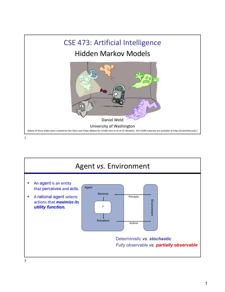
 § An agent is an entity Agent that perceives and acts . Sensors § A rational agent selects Percepts actions that maximize its Environment utility function . ? Actuators Actions Deterministic vs. stochastic Fully observable vs. partially observable 3 1

  2. It’s Hard! Deterministic vs. stochastic Fully observable vs. partially observable 4 Partial Observability in Pacman § A ghost is in the grid somewhere, but Pacman can’t see it! § Sensor readings tell how close a square is to the ghost § On the ghost: red § 1 or 2 away: orange § 2 or 3 away: yellow § 4+ away: green § Sensors are noisy , but we know P(Color | Distance) P(red | 3) P(orange | 3) P(yellow | 3) P(green | 3) Etc. 0.05 0.15 0.5 0.3 5 2

  3. Pacman Maintains a Belief about Ghost Locations Belief = A Probability Distribution over possible locations Visualized here as color density (each ghost has its own color) Four ghosts shown here (not to be confused with colors from sensor readings) 6 Video of Demo Pacman – Sonar (with beliefs) 7 3

  4. PROBABILITY REVIEW 8 8 Random Variables § A random variable is some aspect of the world about which we (may) have uncertainty § R = Is it raining? § T = Is it hot or cold? § D = How long will it take to drive to work? § L = Where is the ghost? § We denote random variables with Capital Letters § Random variables have domains (possible outcomes) § T in {hot, cold} § D in [0, ¥ ) § L in possible locations, maybe {(0,0), (0,1), …} 9 4

  5. Joint Distributions § A joint distribution over a set of random variables: specifies a probability for each assignment (or outcome ): T W P § Must obey: hot sun 0.4 hot rain 0.1 cold sun 0.2 cold rain 0.3 § Number of parameters to specify joint distribution if n variables, each with |domain| = d? § d n -1 For all but the smallest distributions, impractical to write out! 10 Marginal Distributions § Marginal distributions are sub-tables which eliminate variables § Marginalization (summing out): Combine collapsed rows by adding T P hot 0.5 T W P cold 0.5 hot sun 0.4 hot rain 0.1 cold sun 0.2 W P cold rain 0.3 sun 0.6 rain 0.4 11 5

  6. Conditional Probabilities § A simple relation between joint and marginal probabilities § In fact, this is taken as the definition of a conditional probability P(a,b) P(a) P(b) T W P hot sun 0.4 hot rain 0.1 cold sun 0.2 cold rain 0.3 12 Bayes Rule P(coronavirus | sneezing) = ? 0.0000075 P(sneezing | coronavirus) = 0.75 P(sneezing) = 0.10 P(coronavirus) = 0.000001 P(coronavirus | sneezing, in-seattle) = ? 13 13 6

  7. Probability Recap § Conditional probability § Product rule § Chain rule § Bayes rule § X, Y independent if and only if: § X and Y are conditionally independent given Z: if and only if: 14 Conditional Independence S = Smokes cigarettes S / D C = Has (or will have) lung cancer D = Early death S D | C Forall s,d,c P(s,d | c) = P(s | c)*P(d | c) 15 15 7

  8. Probabilistic Inference § Probabilistic inference = “compute a desired probability from other known probabilities (e.g. conditional from joint)” § We generally compute conditional probabilities § P(on time | no reported accidents) = 0.90 § These represent the agent’s beliefs given the evidence § Probabilities change with new evidence: § P(on time | no accidents, 5 a.m.) = 0.95 § P(on time | no accidents, 5 a.m., raining) = 0.80 § Observing new evidence causes beliefs to be updated 16 Outline § Hidden Markov Models (HMMs) § A way to represent a class of probability distributions § Task of Filtering (aka Monitoring) § HMM Forward Algorithm for Filtering § HMM Particle Filter Representation & Algorithm for Filtering § Dynamic Bayes Nets § A generalization & improvement on HMMs 17 17 8

  9. Filtering as “Probabilistic Inference” Stream of observations (evidence) at successive times: e 1 , e 2 , … Important Inference question: P(X t | e 1 , e 2 , … e t ) Deterministic vs. stochastic Fully observable vs. partially observable 18 18 Hidden Markov Models Cool representation for uncertain , sequential data § E.g., ghost locations over time in Pacman § E.g., characters on a line in OCR § E.g., words over time in speech recognition 19 19 9

  10. Hidden Markov Models X 1 X 2 X 3 X 4 X N X 5 E 1 E 2 E 3 E 4 E 5 E N Defines a joint probability distribution: 20 Hidden Markov Model: Example R t-1 P(R t | R t-1 ) P(R 1 ) t 0.7 0.6 f 0.1 R t P(U t | R t ) t 0.9 f 0.2 s c i m a n l § An HMM is defined by: e y d d o n m o n i e t o i v s § Initial distribution: i a n t a a h v r s t r e M y s r M a b § Transitions: o n H o y i t r a a t n S o § Observations: i t a t S Aka “evidence,” “emissions” 21 10

  11. Remember: Joint Distributions § A joint distribution over a set of random variables: specifies a probability for each assignment (or outcome ): T W P § Must obey: hot sun 0.4 hot rain 0.1 cold sun 0.2 cold rain 0.3 § Size of joint distribution if n variables, each with domain sizes d? § d n For all but the smallest distributions, impractical to write out! 22 HMM Joint Distribution for T=100 X 1 E 1 X 2 E 2 X 3 E 3 … X 100 E 100 P T T T T T T T T 0.01 T T T T T T T F 0.007 … F F F F F F F F F 0.026 How Many Parameters? 23 23 11

  12. Umbrella HMM Example: 5 Parameters R t-1 P(R t | R t-1 ) P(R 1 ) t 0.7 0.6 f 0.1 R t P(U t | R t ) t 0.9 f 0.2 s c i m a l n e § An HMM is defined by: y d d o m n o n i t o i § Initial distribution: s e i t n v a a a v h r r t e s y s M § Transitions: r b a M o n H o y r i t a a n t § Observations: S o i t a t S Aka “evidence,” “emissions” 24 Conditional Independence HMMs have two important independence properties: § Future independent of past given the present X t-1 X t+1 | X t ? ? X 1 X 2 X 3 X 4 E 1 E 1 E 3 E 4 Forall x t-1 , x t , x t+1 P(x t-1 , x t+1 | x t ) = P(x t-1 | x t )*P(x t+1 | x t ) 25 12

  13. Conditional Independence HMMs have two important independence properties: § Future independent of past given the present § Current observation independent of all else given current state E t all | X t ? X 1 X 2 X 3 X 4 For example, … E 1 E 1 E 3 E 4 E t X t-1 | X t ? 26 Conditional Independence § HMMs have two important independence properties: § Markov hidden process, future depends on past via the present § Current observation independent of all else given current state X 1 X 2 X 3 X 4 E 1 E 1 E 3 E 4 ? ? § Quiz: does this mean that observations are independent given no evidence? § [ No , correlated by the hidden state, X 2 and X 3 ] 27 13

  14. HMM Computations Given § parameters § evidence E 1:n =e 1:n Inference problems include: § Filtering, find P(X t |e 1:t ) for some t § Most probable explanation, for some t find x* 1:t = argmax x 1:t P(x 1:t |e 1:t ) § Smoothing, find P(X t |e 1:n ) for some t < n 28 Filtering (aka Monitoring) § The task of tracking the agent’s belief state, B(X), over time § B(X) = distribution over world states (outcomes); represents agent knowledge § We start with B(X) in an initial setting, usually uniform § As time passes, or we get evidence/observations, we update B(X) § Many algorithms for this: § Exact probabilistic inference § Particle filter approximation § Kalman filter (a method for handling continuous Real-valued random vars) § invented in the 60’for Apollo Program – real-valued state, Gaussian noise 29 14

  15. Example of HMM Filtering Robot tracking: § States (X) are positions on a map (continuous) § Observations (E) are range readings (continuous) X 1 X 2 X 3 X 4 E 1 E 1 E 3 E 4 30 Example: Robot Localization Example from Michael Pfeiffer Prob 0 1 T=1 Sensor model: never more than 1 mistake Motion model: may not execute action with small prob. 31 15

  16. Example: Robot Localization Green signal = obstacle detected Red signal = no obstacle detected Prob 0 1 At most one error! t=1 32 Example: Robot Localization Prob 0 1 t=2 33 16

  17. Example: Robot Localization Prob 0 1 t=3 34 Example: Robot Localization Prob 0 1 t=4 35 17

  18. Example: Robot Localization Prob 0 1 t=5 36 Other Real HMM Examples § Speech recognition HMMs: § States are specific positions in specific words (so, tens of thousands ) § Observations are acoustic signals (continuous valued) X 1 X 2 X 3 X 4 E 1 E 1 E 3 E 4 37 18

  19. Other Real HMM Examples § Machine translation HMMs: § States are translation options § Observations are words (tens of thousands) X 1 X 2 X 3 X 4 E 1 E 1 E 3 E 4 38 Ghostbusters HMM § X = ghost location: x 11 , … x 33 x 13 x 23 x 33 § Ignore pacman location for now x 12 x 22 x 23 x 11 x 21 x 31 X 1 X 2 X 3 X 4 P(X 1 ) E 1 E 1 E 3 E 4 § How specify HMM? 39 19

Download Presentation
Download Policy: The content available on the website is offered to you 'AS IS' for your personal information and use only. It cannot be commercialized, licensed, or distributed on other websites without prior consent from the author. To download a presentation, simply click this link. If you encounter any difficulties during the download process, it's possible that the publisher has removed the file from their server.

Recommend


More recommend