CSE 473: Artificial Intelligence Hidden Markov Models Daniel Weld - - PDF document

1

CSE 473: Artificial Intelligence Hidden Markov Models

Daniel Weld University of Washington

[Many of these slides were created by Dan Klein and Pieter Abbeel for CS188 Intro to AI at UC Berkeley. All CS188 materials are available at http://ai.berkeley.edu.]

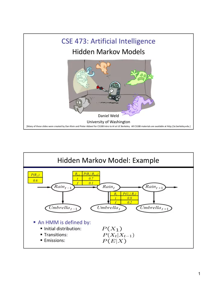
Hidden Markov Model: Example

§ An HMM is defined by:

§ Initial distribution: § Transitions: § Emissions:

P(R1 ) 0.6 Rt-1 t f P(Rt | Rt-1 ) 0.7 0.1 Rt t f P(Ut | Rt ) 0.9 0.2

2

Filtering (aka Monitoring)

§ Filtering, or monitoring, is the task of tracking the distribution B(X) (called “the belief state”) over time § We start with B0(X) in an initial setting, usually uniform § We update Bt(X) computing Bt+1(X)

• 1. As time passes, and

using prob model of how ghosts move

• 2. As we get observations

using prob model of how noisy sensors work

Passage of Time

§ Assume we have current belief P(X | evidence to date) § Then, after one time step passes: § Basic idea: beliefs get “pushed” through the transitions

§ With the “B” notation, we have to be careful about what time step t the belief is about, and what evidence it includes

X2 X1 = X

xt

P(Xt+1, xt|e1:t)

= X

xt

P(Xt+1|xt, e1:t)P(xt|e1:t) = X

xt

P(Xt+1|xt)P(xt|e1:t) § Or compactly:

B0(Xt+1) = X

xt

P(X0|xt)B(xt)

P(Xt+1|e1:t)

3

Observation

§ Assume we have current belief P(X | previous evidence): § Then, after evidence comes in: § Or, compactly:

B0(Xt+1) = P(Xt+1|e1:t) P(Xt+1|e1:t+1) = P(Xt+1, et+1|e1:t)/P(et+1|e1:t) = P(et+1|Xt+1)P(Xt+1|e1:t) = P(et+1|e1:t, Xt+1)P(Xt+1|e1:t)

§ Basic idea: beliefs “reweighted” by likelihood of evidence § Unlike passage of time, we have to normalize

t)/P(et+1|e1:t) t)/P(et+1|e1:t)

+1 P(et+1|Xt+1)B0(Xt+1)

t)/P(et+1|e1:t)

B(Xt+1) =

E1 X1

Defn cond prob Defn cond prob Independence

Observation

§ Assume we have current belief P(X | previous evidence): § Then, after evidence comes in: § Or, compactly: E1 X1

B0(Xt+1) = P(Xt+1|e1:t) P(Xt+1|e1:t+1) = P(Xt+1, et+1|e1:t)/P(et+1|e1:t)

∝Xt+1 P(Xt+1, et+1|e1:t)

= P(et+1|Xt+1)P(Xt+1|e1:t) = P(et+1|e1:t, Xt+1)P(Xt+1|e1:t)

B(Xt+1) ∝Xt+1 P(et+1|Xt+1)B0(Xt+1) § Basic idea: beliefs “reweighted” by likelihood of evidence § Unlike passage of time, we have to renormalize

4

Normalization to Account for Evidence

X E P rain U 0.4 rain

• 0.1

sun U 0.2 sun

• 0.3

X P rain 0.67 sun 0.33 X E P rain U 0.4 sun U 0.2 SELECT the joint probabilities matching the evidence NORMALIZE the selection (make it sum to one)

Since could have seen other evidence, we normalize by dividing by the probability of the evidence we did see (in this case dividing by 0.5)…

Example: Weather HMM

Umbr1 = T Umbr2 = T Rain0 Rain1 Rain2

B(x0=r) = 0.5

P(R1 ) 0.5 Rt-1 t f P(Rt | Rt-1 ) 0.8 0.6 Rt t f P(Ut | Rt ) 0.9 0.3

B’(x1=r) = P(x1=r | x0=r) * 0.5 + P(x1=r | x0=s) * 0.5 = 0.8*0.5 + 0.6*0.5 = 0.7

B0(Xt+1) = X

xt

P(X0|xt)B(xt)

5

Example: Weather HMM

Umbr1 = T Umbr2 = T Rain0 Rain1 Rain2

B(x0=r) = 0.5

P(R1 ) 0.5 Rt-1 t f P(Rt | Rt-1 ) 0.8 0.6 Rt t f P(Ut | Rt ) 0.9 0.3

B’(x1=r) = P(x1=r | x0=r) * 0.5 + P(x1=r | x0=s) * 0.5 = 0.8*0.5 + 0.6*0.5 = 0.7 B(x1=r) ∝ 0.9 * 0.7 = 0.63 B(x1=s) ∝ 0.3 * 0.3 = 0.09 Divide by 0.72 (=0.63+0.09) to normalize B(x1=r) =0.63/0.72 = 0.875

B0(Xt+1) = X

xt

P(X0|xt)B(xt)

B(Xt+1) ∝Xt+1

+1 P(et+1|Xt+1)B0(Xt+1)

Example: Weather HMM

Umbr1 = T Umbr2 = T Rain0 Rain1 Rain2

B(x0=r) = 0.5

P(R1 ) 0.5 Rt-1 t f P(Rt | Rt-1 ) 0.8 0.6 Rt t f P(Ut | Rt ) 0.9 0.3

B0(Xt+1) = X

xt

P(X0|xt)B(xt)

B’(x1=r) = 0.7 B(x1=r) = 0.875 B’(x2=r) = P(x2=r | x1=r)*0.875 + P(x2=r | x1=s)*0.125 = 0.8*0.875 + 0.6*0.125 = 0.775

6

Example: Weather HMM

Umbr1 = T Umbr2 = T Rain0 Rain1 Rain2

B(x0=r) = 0.5

P(R1 ) 0.5 Rt-1 t f P(Rt | Rt-1 ) 0.8 0.6 Rt t f P(Ut | Rt ) 0.9 0.3

B0(Xt+1) = X

xt

P(X0|xt)B(xt)

B’(x1=r) = 0.7 B(x1=r) = 0.875 B’(x2=r) = P(x2=r | x1=r)*0.875 + P(x2=r | x1=s)*0.125 = 0.8*0.875 + 0.6*0.125 = 0.775 B(x1=r) ∝ 0.9 * 0.775 = 0.6975 B(x1=s) ∝ 0.3 * 0.225 = 0.0675 Divide by 0.765 to normalize B(x1=r) = 0.912

B(Xt+1) ∝Xt+1

+1 P(et+1|Xt+1)B0(Xt+1)

Particle Filtering

7

Particle Filtering Overview

§ Approximation technique to solve filtering problem § Represents P distribution with samples § Filtering still operates in two steps

§ Elapse time § Incorporate observations

§ (But this part has two sub-steps: weight & resample)

38

Particle Filtering

§ Sometimes |X| is too big to use exact inference

§ |X| may be too big to even store B(X) § E.g. X is continuous

§ Solution: approximate inference

§ Track samples of X, not exact distribution of values § Samples are called particles § Time per step is linear in the number of samples § But: number needed may be large § In memory: list of particles, not states

§ Particle is just new name for sample § This is how robot localization works in practice

8

Remember…

An HMM is defined by:

§ Initial distribution: § Transitions: § Emissions:

Here’s a Single Particle

§ It represents a hypothetical state where the robot is in (1,2)

9

Particles Approximate Distribution

§ Our representation of P(X) is now a list of N particles (samples)

§ Generally, N << |X| Particles: (3,3) (2,3) (3,3) (3,2) (3,3) (3,2) (1,2) (3,3) (3,3) (2,3) P(x) Distribution P(x=<3,3>) = 5/10 = 50%

Particle Filtering

A more compact view overlays the samples:

Encodes à

0.0 0.2 0.1 0.0 0.5 0.2 0.0 0.2 0.5

10 P(x) Distribution

Another Example

In the weather HMM, suppose we decide to approximate the distributions with 5 particles. To initialize the filter, we draw 5 samples from B(x0=r) = 0.5 and we might get the following set of particles:

44

Not such a good approximation, but that’s life.

Particles: S R R S S

Representation: Particles

§ Our representation of P(X) is now a list of N particles (samples)

§ Generally, N << |X| § Storing map from X to counts would defeat the purpose

§ P(x) approximated by (number of particles with value x) / N

§ More particles, more accuracy

§ What is P((2,2))?

§ In fact, many x may have P(x) = 0!

Particles: (3,3) (2,3) (3,3) (3,2) (3,3) (3,2) (1,2) (3,3) (3,3) (2,3)

0/10 = 0%

11

Particle Filtering Algorithm

• 1. Elapse Time
• 2. Observe
• 2a. Downweight samples based on evidence
• 2b. Resample

47

Particle Filtering: Elapse Time

§ For each particle, x, move x by sampling its next position from the transition model

§ This is like prior sampling – samples’ frequencies reflect the transition probabilities § Here, most samples move clockwise, but some move in another direction or stay in place

§ This captures the passage of time

§ If enough samples, close to exact values before and after (consistent)

Particles: (3,3) (2,3) (3,3) (3,2) (3,3) (3,2) (1,2) (3,3) (3,3) (2,3) Particles: (3,2) (2,3) (3,2) (3,1) (3,3) (3,2) (1,3) (2,3) (3,2) (2,2)

Aka: sample(P(xt+1 | xt))

12

§ Slightly trickier:

§ Don’t sample observation, fix it § Similar to likelihood weighting, § For each particle, x, down-weight x based on the evidence § As before, the probabilities don’t sum to

• ne, since all have been downweighted

(in fact they now sum to (N times) an approximation of P(e))

Particle Filtering: Observe

Particles: (3,2) w=.9 (2,3) w=.2 (3,2) w=.9 (3,1) w=.4 (3,3) w=.4 (3,2) w=.9 (1,3) w=.1 (2,3) w=.2 (3,2) w=.9 (2,2) w=.4 Particles: (3,2) (2,3) (3,2) (3,1) (3,3) (3,2) (1,3) (2,3) (3,2) (2,2)

Particle Filtering Observe Part II: Resample

§ Rather than tracking weighted samples, we resample § N times, we choose from our weighted sample distribution (i.e. draw with replacement)

Particles: (3,2) w=.9 (2,3) w=.2 (3,2) w=.9 (3,1) w=.4 (3,3) w=.4 (3,2) w=.9 (1,3) w=.1 (2,3) w=.2 (3,2) w=.9 (2,2) w=.4 (New) Particles: (3,2) (2,2) (3,2) (2,3) (3,3) (3,2) (3,1) (3,2) (3,1) (3,2)

§ This is equivalent to renormalizing the distribution § Now the update is complete for this time step, continue with the next one

(3,2) (2,3) (3,2)

w=.9 w=.2 w=.9

(2,2)

w=.4

Draw random number in [0, 5.3]

13

Recap: Particle Filtering

§ Particles: track samples of states rather than an explicit distribution

Particles: (3,3) (2,3) (3,3) (3,2) (3,3) (3,2) (1,2) (3,3) (3,3) (2,3)

Elapse Weight Resample

Particles: (3,2) (2,3) (3,2) (3,1) (3,3) (3,2) (1,3) (2,3) (3,2) (2,2) Particles: (3,2) w=.9 (2,3) w=.2 (3,2) w=.9 (3,1) w=.4 (3,3) w=.4 (3,2) w=.9 (1,3) w=.1 (2,3) w=.2 (3,2) w=.9 (2,2) w=.4 (New) Particles: (3,2) (2,2) (3,2) (2,3) (3,3) (3,2) (1,3) (2,3) (3,2) (3,2)

[Demos: ghostbusters particle filtering (L15D3,4,5)]

Video of Demo – Moderate Number of Particles

Uniform initialization (!) Circular dynamics

14

Video of Demo – One Particle

Uniform initialization (ha!) Circular dynamics

Video of Demo – Huge Number of Particles

Actually looks uniform ! but look closely Circular dynamics

15

Robot Localization

§ In robot localization:

§ We know the map, but not the robot’s position § Observations may be vectors of range finder readings § State space and readings are typically continuous (works basically like a very fine grid) and so we cannot store B(X) § Particle filtering is a main technique

Particle Filter Localization (Sonar)

[Video: global-sonar-uw-annotated.avi]

16

Particle Filter Localization (Laser)

[Video: global-floor.gif]

Robot Mapping

§ SLAM: Simultaneous Localization And Mapping

§ We do not know the map or our location § State consists of position AND map! § Main techniques: Kalman filtering (Gaussian HMMs) and particle methods

DP-SLAM, Ron Parr [Demo: PARTICLES-SLAM-mapping1-new.avi]

17

Particle Filter SLAM – Video 1

[Demo: PARTICLES-SLAM-mapping1-new.avi]

Particle Filter SLAM – Video 2

[Demo: PARTICLES-SLAM-fastslam.avi]