Orthogonal projections of row spaces P B denotes the operator that - - PowerPoint PPT Presentation

Orthogonal projections of row spaces

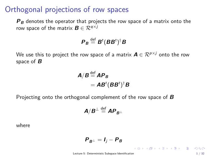
PB denotes the operator that projects the row space of a matrix onto the row space of the matrix B ∈ Rq×j PB

def

= Bt(BBt)†B We use this to project the row space of a matrix A ∈ Rp×j onto the row space of B A/B

def

= APB = ABt(BBt)†B Projecting onto the orthogonal complement of the row space of B A/B⊥ def = APB⊥ where PB⊥ = Ij − PB

Lecture 5: Deterministic Subspace Identification 1 / 32

Orthogonal projections of row spaces

We can decompose A as A = APB + APB⊥ Alternatively, we can decompose A as a linear combination of rows of B and rows of the orthogonal complement of B using LBB

def

= A/B LB⊥B⊥ def = A/B⊥ and find A = LBB + LB⊥B⊥

Lecture 5: Deterministic Subspace Identification 2 / 32

Oblique projections of row spaces

Decomposition of A as linear combinations of two non-orthogonal matrices B and C and the orthogonal complement of B and C A = LBB + LCC + LB⊥,C⊥

• B

C ⊥ where LCC is defined as the oblique projection of the row space of A along the row space of B on the row space of C A/CB

def

= LCC

B A/BC A C

Lecture 5: Deterministic Subspace Identification 3 / 32

Oblique projections of row spaces

How to decompose?

• 1. Project A on joint row space of B and C

A/ C B

• = A

Ct Bt CCt CBt BCt BBt † C B

• 2. Decompose along row spaces of B and B

Definition 1 (Oblique projections).

The oblique projection of the row space of A ∈ Rp×j along the row space

• f B ∈ Rq×j on the row space of C ∈ Rr×j is defined as

A/BC

def

= A

• Ct

Bt CCt CBt BCt BBt †

first r columns

C Properties B/CB = 0 C/CB = C

Lecture 5: Deterministic Subspace Identification 4 / 32

Oblique projections of row spaces

Corollary 2 (Oblique projections).

The oblique projection of the row space of A ∈ Rp×j along the row space

• f B ∈ Rq×j on the row space of C ∈ Rr×j can also be defined as

A/BC = [A/B⊥] · [C/B⊥]† · C

B B⊥ A/BC A C

Lecture 5: Deterministic Subspace Identification 5 / 32

Principal angles and directions

The principal angles between two subspaces are a generalization of an angle between two vectors

a1 = b1 θ1 = 0 a2 b2 θ2

Lecture 5: Deterministic Subspace Identification 6 / 32

Principal angles and directions

Definition 3 (Principal angles and directions).

The principal angles θ1 ≤ θ2 ≤ . . . ≤ π/2 between the row spaces of A and B of two matrices A ∈ Rp×j and B ∈ Rq×j and the corresponding principal directions ai ∈ row space A and bi ∈ row space B are defined recursively as: cos θk = max

a ∈ row space A, b ∈ row space B

atb subject to a = b = 1 and for k > 1, atai = 0 for i = 1, . . . , k − 1 and btbi = 0 for i = 1, . . . , k − 1.

Lecture 5: Deterministic Subspace Identification 7 / 32

Principal angles and directions

Given two matrices A ∈ Rp×j and B ∈ Rq×j and the singular value decomposition: At(AAt)†ABt(BBt)†B = USV t then the principal directions between the row spaces of A and B are equal to the rows of Ut and the rows of V t. The cosines of the principal angles between the row spaces of A and B are defined as the singular values (the diagonal of S). The principal directions and angles between the row spaces of A and B are denoted as: [A ∢ B]

def

= Ut [A ∢ B]

def

= V t [A ∢ B]

def

= S

Lecture 5: Deterministic Subspace Identification 8 / 32

Principal angles and directions

The principal angles and directions between the row spaces of A and B

• f two matrices A ∈ Rp×j and B ∈ Rq×j can also be found through the

singular value decomposition of

• AAt−1/2

ABt BBt−1/2 = USV t as: [A ∢ B]

def

= Ut AAt−1/2 A [A ∢ B]

def

= V t BBt−1/2 B [A ∢ B]

def

= S

Lecture 5: Deterministic Subspace Identification 9 / 32

Part I Deterministic Subspace Identification

Lecture 5: Deterministic Subspace Identification 10 / 32

Deterministic identification problem

Given: s measurements of the input uk ∈ Rm and the output yk ∈ Rl generated by the unknown deterministic system of order n: dk+1 = Adk + Buk yk = Cdk + Duk Determine:

◮ The order n of the unknown system. ◮ The system matrices A ∈ Rn×n, B ∈ Rn×m, C ∈ Rl×n, D ∈ Rl×m

(up to within a similarity transformation).

Lecture 5: Deterministic Subspace Identification 11 / 32

Block Hankel matrices

U0|2i−1

def

=                u0 u1 u2 . . . uj−1 u1 u2 u3 . . . uj . . . . . . ui−1 ui ui+1 . . . ui+j−2 ui ui+1 ui+2 . . . ui+j−1 ui+1 ui+2 ui+3 . . . ui+j . . . . . . u2i−1 u2i u2i+1 . . . u2i+j−2                =

• U0|i−1

Ui|2i−1

• =
• Up

Uf

• Lecture 5: Deterministic Subspace Identification

12 / 32

Block Hankel matrices

Block Hankel matrix dimensions

◮ For i block rows and uk ∈ Rm, the number of rows in U0|2i−1

equals 2mi.

◮ For s measurement, the number of columns j is typically equal to

s − 2i + 1. Subscript p stands for “past” and subscript f stands for “future”. The matrices Up (the past inputs) and Uf (the future inputs) are defined by splitting U0|2i−1 in two equal parts of i block rows. Corresponding columns of Up and Uf have no elements in common, thus the distinction between past and future.

Lecture 5: Deterministic Subspace Identification 13 / 32

Block Hankel matrices

Distinction between past and future? U0|2i−1

def

=                u0 u1 u2 . . . uj−1 u1 u2 u3 . . . uj . . . . . . ui−1 ui ui+1 . . . ui+j−2 ui ui+1 ui+2 . . . ui+j−1 ui+1 ui+2 ui+3 . . . ui+j . . . . . . u2i−1 u2i u2i+1 . . . u2i+j−2                =

• U0|i

Ui+1|2i−1

• =
• U+

p

U−

f

• Note that U+

p has i + 1 block rows, whereas U− p only has i − 1 block

rows.

Lecture 5: Deterministic Subspace Identification 14 / 32

Input-output data matrices

W 0|i−1

def

=

• U0|i−1

Y 0|i−1

• =

Up Y p

• = W p

where Y p is defined in a similar way to Up. Or for a shifted boundary: W +

p =

U+

p

Y +

p

• Lecture 5: Deterministic Subspace Identification

15 / 32

Notation

We denote the state sequence matrix by Xd

i def

= di di+1 . . . di+j−2 di+j−1

• ∈ Rn×j

The observability matrix Γi

def

=       C CA CA2 . . . CAi−1       ∈ Rli×n Reversed controllability matrix ∆i[d]

def

=

• Ai−1B

Ai−2B . . . AB B

• ∈ Rn×mi

Lecture 5: Deterministic Subspace Identification 16 / 32

Notation

Block Toeplitz with Markov parameters Hd

i def

=        D . . . CB D CAB CB D . . . . . . CAi−2B CAi−3B CAi−4B . . . D        ∈ Rli×mi

Lecture 5: Deterministic Subspace Identification 17 / 32

Matrix input-output equations

Y p = ΓiXd

p + Hd i Up

Y f = ΓiXd

f + Hd i Uf

Xd

f = AiXd p + ∆i[d]Up

Hd

i Uf

ΓiXd

f

Y f

Lecture 5: Deterministic Subspace Identification 18 / 32

Subspace Theorem for Deterministic Identification

Let

◮ uk be persistently excited of order 2i (i.e. rank U0|2i−1 = 2mi ◮ R ((Uf )t) ∩ R

• (Xd

p)t

= {0}

◮ W 1 ∈ Rli×li, W 2 ∈ Rj×j are weighting matrices, with

rank (W 1) = li and rank (W p) = rank (W pW 2) Let Oi

def

= Y f /Uf W p and W 1OiW 2 = U1 U2 S1 V t

1

V t

2

• = U1S1V t

1

then Oi = ΓiXd

f

n = #(σi = 0) Γi = W −1

1 U1S1/2 1

T Xd

f W 2 = T −1S1/2 1

V t

1

Xd

f = Γ† i Oi

Lecture 5: Deterministic Subspace Identification 19 / 32

Subspace Theorem for Deterministic Identification

Oi = ΓiXd

f

Hd

i Uf

Y f W p rank (Y f /Uf W p) = n row space (Y f /Uf W p) = row space (Xd

f )

column space (Y f /Uf W p) = column space (Γi)

Lecture 5: Deterministic Subspace Identification 20 / 32

Rank deficiency & LTI systems

If uk is persistently exciting of order i, i.e. rank

• U0|i−1
• = mi

then rank

• W 0|i−1
• = rank

U0|i−1 Y 0|i−1

• = mi + n

Proof follows from matrix input-output equation:

• Ili

−Hd

i

Imi Y p Up

• =

Γi Imi Xd

p

Up

• Lecture 5: Deterministic Subspace Identification

21 / 32

Intersection algorithm

If uk is persistently exciting of order 2i, then rank

• W 0|i−1
• = mi + n

rank

• W i|2i−1
• = mi + n

rank

• W 0|2i−1
• = 2mi + n

Also note that W 0|2i−1 = W 0|i−1 W i|2i−1

• Apply Grassmann:

dim R

• W t

0|i−1

• ∩ R
• W t

i|2i−1

• = (mi + n) + (mi + n) − (2mi + n) = n

So: n-dimensional intersection between ‘past’ and ‘future’! dim R

• W t

0|i−1

• ∩ R
• W t

i|2i−1

• = R
• (Xd

p)t

Lecture 5: Deterministic Subspace Identification 22 / 32

Intersection algorithm

dim R

• W t

0|i−1

• ∩ R
• W t

i|2i−1

• = R
• (Xd

p)t

Proof: Xd = Γ†

i Y f /Uf W p

and Xd

f = Γ† i Y f − Γ† i Hd i Uf

Lecture 5: Deterministic Subspace Identification 23 / 32

Projection algorithm

Y f = ΓiXd

f + Hd i Uf =

⇒ Y f /U⊥

f = ΓiXd f /U⊥ f

Hence R

• Y f /U⊥

f

• = R (Γi)

n = rank

• Y f /U⊥

f

• Compare to the deterministic subspace theorem with

W 1 = Ili W 2 = PU⊥

f Lecture 5: Deterministic Subspace Identification 24 / 32

Projection algorithm

Calculate using the LQ-decomposition Uf Y f

• =

R11 R21 R22 Qt

1

Qt

2

• Hence

Uf = R11Qt

1

Y f = R21Qt

1 + R22Qt 2

so that Y f /U⊥

f = R22Qt 2

rank (R22) = n R (R22) = R (Γi) Observe: only need R to find Γi and n!

Lecture 5: Deterministic Subspace Identification 25 / 32

How to compute system matrices?

Case 1: via the states Can be shown: Oi−1

def

= Y −

f /U−

f W +

p

= Γi−1Xd

i+1

Also: Γi−1 = Γi Hence: Xd

i+1 = Γ† i−1Oi−1

• Xd

i+1

Y i|i

• known

= A B C D Xd

i

Ui|i

• known

Lecture 5: Deterministic Subspace Identification 26 / 32

Deterministic algorithm 1 (via the states)

Data: Data matrices U0|2i−1, Y 0|2i−1 Result: System matrices A, B, C and D begin Calculate the oblique projections Oi = Y f /Uf W p Oi−1 = Y −

f /U−

f W +

p

Compute SVD of weighted oblique projection W 1OiW 2 = USV t Determine system order n from S, partition accordingly for U1 and S1 Determine Γi and Γi−1 as Γi = W −1

1 U1S1/2 1

Γi−1 = Γi end

Lecture 5: Deterministic Subspace Identification 27 / 32

Deterministic algorithm 1 (via the states) cont.

Data: Data matrices U0|2i−1, Y 0|2i−1 Result: System matrices A, B, C and D begin Determine Xd

i and Xd i+1 as

Xd

i = Γ† i Oi

Xd

i+1 = Γ† i−1Oi−1

Solve for A, B, C and D

• Xd

i+1

Y i|i

• =
• A

B C D Xd

i

Ui|i

• end

Lecture 5: Deterministic Subspace Identification 28 / 32

How to compute system matrices?

Case 2: using the observability matrix Matrices A and C follow from the shift structure of Γi: ΓiA = Γi Matrices B and D follow from: Γ⊥

i Y f = Γ⊥ i Hd i Uf =

⇒ Γ⊥

i Y f U† f

• ∈R(li−n)×mi

= Γ⊥

i

• ∈R(li−n)×li

Hd

i

• ∈Rli×mi

can be expressed as

• M1

M2 . . . Mi

• =
• L1

L2 . . . Li

• ×

       D . . . CB D . . . CAB CB D . . . . . . . . . CAi−2B CAi−3B CAi−4B . . . D        (1)

Lecture 5: Deterministic Subspace Identification 29 / 32

How to compute system matrices?

Obtain B and D by solving the linear system      M1 M2 . . . Mi     

∈Ri(li−n)×m

=        L1 L2 . . . Li−1 Li L2 L3 . . . Li L3 L4 . . . . . . . . . Li . . .       

• ∈Ri(li−n)×li

Il Γi

• ∈Rli×(l+n)

D B

• Lecture 5: Deterministic Subspace Identification

30 / 32

Deterministic algorithm 2 (using the observ. matrix)

Data: Data matrices U0|2i−1, Y 0|2i−1 Result: System matrices A, B, C and D begin Calculate the oblique projection Oi = Y f /Uf W p Compute SVD of weighted oblique projection W 1OiW 2 = USV t Determine system order n from S, partition accordingly for U1 and S1 Determine Γi and Γ⊥

i

as Γi = W −1

1 U1S1/2 1

Γ⊥

i = Ut 2W 1

end

Lecture 5: Deterministic Subspace Identification 31 / 32

Deterministic algorithm 2 (using the observ. matrix) cont.

Data: Data matrices U0|2i−1, Y 0|2i−1 Result: System matrices A, B, C and D begin Compute A and C as A = Γi

†Γi

C = first l rows of Γi Solve B and D from Γ⊥

i Y f U† f = Γ⊥ i Hd i

end

Lecture 5: Deterministic Subspace Identification 32 / 32