Non-Deterministic Search CS 188: Artificial Intelligence Markov - PDF document

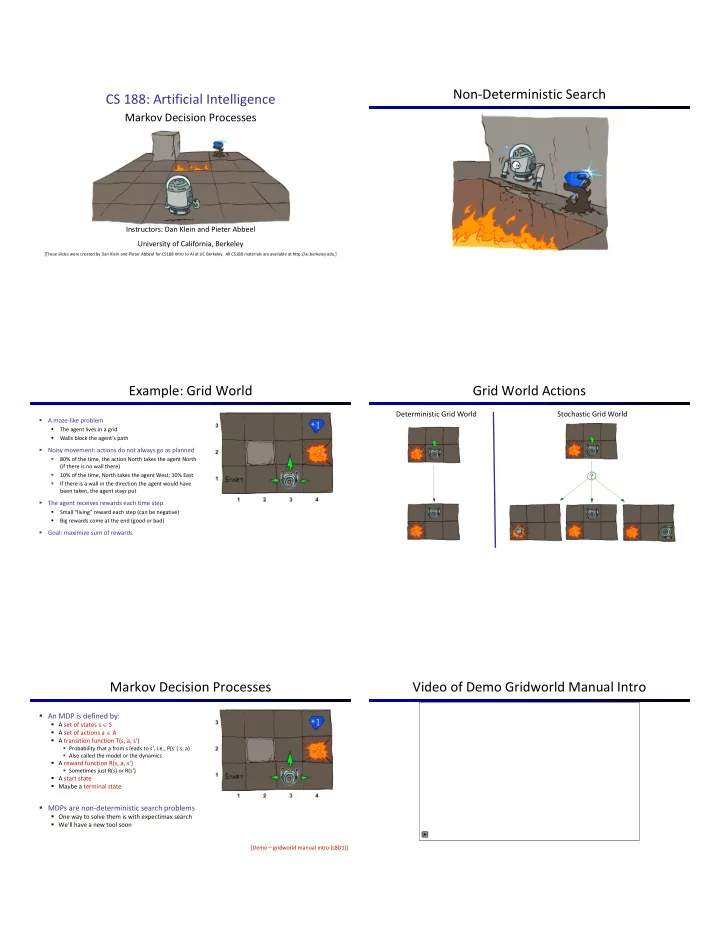
Non-Deterministic Search CS 188: Artificial Intelligence Markov Decision Processes Instructors: Dan Klein and Pieter Abbeel University of California, Berkeley [These slides were created by Dan Klein and Pieter Abbeel for CS188 Intro to AI at UC Berkeley. All CS188 materials are available at http://ai.berkeley.edu.] Example: Grid World Grid World Actions Deterministic Grid World Stochastic Grid World � A maze-like problem � The agent lives in a grid � Walls block the agent’s path � Noisy movement: actions do not always go as planned � 80% of the time, the action North takes the agent North (if there is no wall there) � 10% of the time, North takes the agent West; 10% East � If there is a wall in the direction the agent would have been taken, the agent stays put � The agent receives rewards each time step � Small “living” reward each step (can be negative) � Big rewards come at the end (good or bad) � Goal: maximize sum of rewards Markov Decision Processes Video of Demo Gridworld Manual Intro � An MDP is defined by: � A set of states s ∈ S � A set of actions a ∈ A � A transition function T(s, a, s’) � Probability that a from s leads to s’, i.e., P(s’| s, a) � Also called the model or the dynamics � A reward function R(s, a, s’) � Sometimes just R(s) or R(s’) � A start state � Maybe a terminal state � MDPs are non-deterministic search problems � One way to solve them is with expectimax search � We’ll have a new tool soon [Demo – gridworld manual intro (L8D1)]

What is Markov about MDPs? Policies � “Markov” generally means that given the present state, the � In deterministic single-agent search problems, future and the past are independent we wanted an optimal plan, or sequence of actions, from start to a goal � For Markov decision processes, “Markov” means action outcomes depend only on the current state � For MDPs, we want an optimal policy π *: S → A � A policy π gives an action for each state � An optimal policy is one that maximizes expected utility if followed Andrey Markov � An explicit policy defines a reflex agent (1856-1922) Optimal policy when R(s, a, s’) = -0.03 for all non-terminals s � Expectimax didn’t compute entire policies � This is just like search, where the successor function could only � It computed the action for a single state only depend on the current state (not the history) Optimal Policies Example: Racing R(s) = -0.01 R(s) = -0.03 R(s) = -0.4 R(s) = -2.0 Example: Racing Racing Search Tree � A robot car wants to travel far, quickly � Three states: Cool, Warm, Overheated � Two actions: Slow , Fast 0.5 +1 � Going faster gets double reward 1.0 Fast Slow -10 +1 0.5 Warm Slow Fast 0.5 +2 Cool 0.5 +1 Overheated 1.0 +2

MDP Search Trees Utilities of Sequences � Each MDP state projects an expectimax-like search tree s is a state s a (s, a) is a s, a q-state (s,a,s ’ ) called a transition T(s,a,s ’ ) = P(s ’ |s,a) s,a,s ’ R(s,a,s ’ ) s ’ Utilities of Sequences Discounting � It’s reasonable to maximize the sum of rewards � What preferences should an agent have over reward sequences? � It’s also reasonable to prefer rewards now to rewards later � One solution: values of rewards decay exponentially � More or less? [1, 2, 2] or [2, 3, 4] � Now or later? [0, 0, 1] or [1, 0, 0] Worth Now Worth Next Step Worth In Two Steps Discounting Stationary Preferences � Theorem: if we assume stationary preferences: � How to discount? � Each time we descend a level, we multiply in the discount once � Why discount? � Sooner rewards probably do have higher utility than later rewards � Also helps our algorithms converge � Then: there are only two ways to define utilities � Example: discount of 0.5 � Additive utility: � U([1,2,3]) = 1*1 + 0.5*2 + 0.25*3 � U([1,2,3]) < U([3,2,1]) � Discounted utility:

Quiz: Discounting Infinite Utilities?! � Problem: What if the game lasts forever? Do we get infinite rewards? � Given: � Solutions: � Actions: East, West, and Exit (only available in exit states a, e) � Finite horizon: (similar to depth-limited search) � Transitions: deterministic � Terminate episodes after a fixed T steps (e.g. life) � Gives nonstationary policies ( π depends on time left) � Quiz 1: For γ = 1, what is the optimal policy? � Discounting: use 0 < γ < 1 � Quiz 2: For γ = 0.1, what is the optimal policy? � Smaller γ means smaller “horizon” – shorter term focus � Quiz 3: For which γ are West and East equally good when in state d? � Absorbing state: guarantee that for every policy, a terminal state will eventually be reached (like “overheated” for racing) Recap: Defining MDPs Solving MDPs � Markov decision processes: s � Set of states S � Start state s 0 a � Set of actions A s, a � Transitions P(s’|s,a) (or T(s,a,s’)) s,a,s ’ � Rewards R(s,a,s’) (and discount γ ) s ’ � MDP quantities so far: � Policy = Choice of action for each state � Utility = sum of (discounted) rewards Optimal Quantities Snapshot of Demo – Gridworld V Values � The value (utility) of a state s: V * (s) = expected utility starting in s and s is a s state acting optimally a (s, a) is a � The value (utility) of a q-state (s,a): s, a q-state Q * (s,a) = expected utility starting out s,a,s’ (s,a,s’) is a having taken action a from state s and transition (thereafter) acting optimally s’ � The optimal policy: π * (s) = optimal action from state s Noise = 0.2 Discount = 0.9 [Demo – gridworld values (L8D4)] Living reward = 0

Snapshot of Demo – Gridworld Q Values Values of States � Fundamental operation: compute the (expectimax) value of a state � Expected utility under optimal action s � Average sum of (discounted) rewards � This is just what expectimax computed! a s, a � Recursive definition of value: s,a,s ’ s ’ Noise = 0.2 Discount = 0.9 Living reward = 0 Racing Search Tree Racing Search Tree Racing Search Tree Time-Limited Values � We’re doing way too much � Key idea: time-limited values work with expectimax! � Define V k (s) to be the optimal value of s if the game ends in k more time steps � Problem: States are repeated � Equivalently, it’s what a depth-k expectimax would give from s � Idea: Only compute needed quantities once � Problem: Tree goes on forever � Idea: Do a depth-limited computation, but with increasing depths until change is small � Note: deep parts of the tree eventually don’t matter if γ < 1 [Demo – time-limited values (L8D6)]

k=0 k=1 Noise = 0.2 Noise = 0.2 Discount = 0.9 Discount = 0.9 Living reward = 0 Living reward = 0 k=2 k=3 Noise = 0.2 Noise = 0.2 Discount = 0.9 Discount = 0.9 Living reward = 0 Living reward = 0 k=4 k=5 Noise = 0.2 Noise = 0.2 Discount = 0.9 Discount = 0.9 Living reward = 0 Living reward = 0

k=6 k=7 Noise = 0.2 Noise = 0.2 Discount = 0.9 Discount = 0.9 Living reward = 0 Living reward = 0 k=8 k=9 Noise = 0.2 Noise = 0.2 Discount = 0.9 Discount = 0.9 Living reward = 0 Living reward = 0 k=10 k=11 Noise = 0.2 Noise = 0.2 Discount = 0.9 Discount = 0.9 Living reward = 0 Living reward = 0

k=12 k=100 Noise = 0.2 Noise = 0.2 Discount = 0.9 Discount = 0.9 Living reward = 0 Living reward = 0 Computing Time-Limited Values Value Iteration Value Iteration Example: Value Iteration � Start with V 0 (s) = 0: no time steps left means an expected reward sum of zero � Given vector of V k (s) values, do one ply of expectimax from each state: V k+1 (s) 3.5 2.5 0 a s, a � Repeat until convergence s,a,s ’ 2 1 0 V k (s’) � Complexity of each iteration: O(S 2 A) Assume no discount! 0 0 0 � Theorem: will converge to unique optimal values � Basic idea: approximations get refined towards optimal values � Policy may converge long before values do

Convergence* Next Time: Policy-Based Methods � How do we know the V k vectors are going to converge? � Case 1: If the tree has maximum depth M, then V M holds the actual untruncated values � Case 2: If the discount is less than 1 � Sketch: For any state V k and V k+1 can be viewed as depth k+1 expectimax results in nearly identical search trees � The difference is that on the bottom layer, V k+1 has actual rewards while V k has zeros � That last layer is at best all R MAX � It is at worst R MIN � But everything is discounted by γ k that far out � So V k and V k+1 are at most γ k max|R| different � So as k increases, the values converge