[PPT] - The k -variance problem Orthogonal projections If V R d , then V PowerPoint Presentation

SLIDE 1

The k-variance problem Orthogonal projections

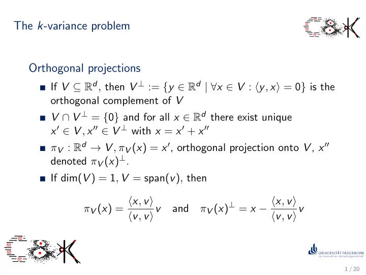
If V ⊆ Rd, then V ⊥ := {y ∈ Rd | ∀x ∈ V : y, x = 0} is the

rthogonal complement of V

V ∩ V ⊥ = {0} and for all x ∈ Rd there exist unique x′ ∈ V , x′′ ∈ V ⊥ with x = x′ + x′′ πV : Rd → V , πV (x) = x′, orthogonal projection onto V , x′′ denoted πV (x)⊥. If dim(V ) = 1, V = span(v), then πV (x) = x, v v, vv and πV (x)⊥ = x − x, v v, vv

1 / 20

SLIDE 2

The k-variance problem Problem 5.1 (k-variance problem)

Given P ⊂ Rd, |P| = n and k ∈ N, Find the k-dimensional subspace Vk that minimizes D(P, V ) :=

p∈P

p − πV (p)2. The subspace Vk is called the (k-dimensional) singular value decomposition of P.

2 / 20

SLIDE 3

Characterization of optimal subspace Lemma 5.2

For all P ⊂ Rd Vk = argminV :dim(V )=k{D(P, V )} ⇔ Vk = argmaxV :dim(V )=k   

p∈P

πV (p)2    . More generally, for every subspace V ⊆ Rd D(P, V ) =

q∈P

q2 −

q∈P

πV (q)2.

3 / 20

SLIDE 4

Complexity and relation to k-means Theorem 5.3

For every P ⊂ Rd and k ∈ N the subspace Vk minimizing D(P, V ) can be computed efficiently.

Lemma 5.4

For every P ⊂ Rd and k ∈ N D(P, Vk) ≤ optk(P).

4 / 20

SLIDE 5

Spectral algorithms Spectral algorithms

Given P ⊂ Rd,

1 compute the singular value decomposition Vk, i.e. the

subspace minimizing D(P, V ),

2 solve your favorite clustering problem with your favorite

algorithm on input πVk(P) := {πVk(p) : p ∈ P},

3 return the solution found in the previous step.

5 / 20

SLIDE 6

Orthonormal bases Definition 5.5

Let V ⊆ Rd be a k-dimensional subspace of Rd and let B = {v1, . . . , vk} be a basis of V . Basis B is an orthonormal basis (ONB) of V if

1 vi = 1, i = 1, . . . , k 2 vi, vj = 0 for i = j, i, j = 1, . . . , n.

Theorem 5.6

Every subspace V ⊆ Rd has an orthonormal basis. Moreover, any

rthonormal basis of V can be extended to an orthonormal basis of

Rd.

6 / 20

SLIDE 7

Length-preserving linear maps

V ⊆ Rd subspace with orthonormal basis BV = {v1, . . . , vk}. U ∈ Rk×d matrix with rows vT

1 , . . . , vT k .

ΠV denotes function ΠV : Rd → Rk, x → U · x

Theorem 5.7

The linear function ΠV has the following properties:

1 ΠV is surjective. 2 ΠV is length-preserving on V , i.e. for all

x ∈ V : x = ΠV (x).

7 / 20

SLIDE 8

Spectral algorithms revisited Spectral algorithms

Given P ⊂ Rd,

1 compute the singular value decomposition Vk, i.e. the

subspace minimizing D(P, V ),

2 solve your favorite clustering problem with your favorite

algorithm on input πVk(P) := {πVk(p) : p ∈ P}, i.e. compute an orthonormal basis for Vk and apply your favorite clustering algorithm on the set ΠVk(πVk(P))

3 return the solution found in the previous step.

8 / 20

SLIDE 9

k-variance and k-means Lemma 5.8

Let P ⊂ Rd and let V be an arbitrary k-dimensional subspace of

Rd. Then
ptk(πV (P)) ≤ optk(P),

where optk(P) denotes the cost of an optimal solution of k-means with input P.

9 / 20

SLIDE 10

k-variance and k-means Lemma 5.9

Let P ⊂ Rd and let V be an arbitrary k-dimensional subspace of

Rd. Assume ˆ

C = { ˆ C1, . . . , ˆ Ck} is a k-clustering of πV (P) and denote by C := {C1, . . . , Ck} with Ci := {p ∈ P : πV (p) ∈ ˆ Ci}, the corresponding k-clustering of P. Then cost(πV (P), ˆ C) ≤ cost(P, C) ≤ cost(πV (P), ˆ C) + D(P, V ).

10 / 20

SLIDE 11

Approximation guarantees for spectral algorithms Spectral algorithms

Given P ⊂ Rd,

1 compute the singular value decomposition Vk, i.e. the

subspace minimizing D(P, C),

2 solve your favorite clustering problem with your favorite

algorithm on input πVk(P) := {πVk(p) : p ∈ P},

3 return the solution found in the previous step.

Theorem 5.10

Let P ⊂ Rd and let Vk be the k-dimensional subspace of Rd minimizing D(P, V ). If ˆ C is a γ-approximate k-clustering for πVk(P), then the corresponding k-clustering C as defined in the previous lemma is a (γ + 1)-approximate k-clustering for P.

11 / 20

SLIDE 12

An excact algorithm for k-means

Exact-k-Means(P, k)

Compute the set K of sets of t hyperplanes with k ≤ t ≤ k

2

where each

hyperplane contains d affinely independent points from P; for S ∈ K do check that S defines an arrangement of exactly k cells; for all assignments aS of points of P on hyperplanes in S to cells do for all cells do compute the centroid of points of P in the cell; end CS,as := set of centroids computed in the previous step; end CS := argminCS,aS {D(P, CS,aS )}; end return argminCS {D(P, CS)};

12 / 20

SLIDE 13

An excact algorithm for k-means Theorem 5.11

Algorithm Exact-k-Means solves the k-means problem

ptimally in time O
ndk2/2

.

13 / 20

SLIDE 14

A spectral approximation algorithm

Spectral-k-Means(P, k) Compute Vk := argminV :dim(V )=k{D(P, V )}; ¯ C := Exact-k-Means(πVk(P), k); return ¯ C;

Theorem 5.12

Spectral-k-Means is an approximation algorithm for the k-means problem with running time O

n · d2 + nk3/2

and approximation factor 2.

14 / 20

SLIDE 15

Matrix representation of point sets

P = {p1, . . . , pn} ⊂ Rd matrix A ∈ Rd×n with columns pi called matrix representation

f P

rows of AT ∈ Rn×d are pT

i

for every v ∈ Rd:

AT · v = (p1, v, . . . , pn, v)T ∈ Rn AT · v2 = v T · A · AT · v = n

i=1pi, v2

15 / 20

SLIDE 16

Characterization of k-variance solutions Theorem 5.13

For every set of points P ⊂ Rd, |P| = n, with matrix representation A ∈ Rd×n : argmaxV :dim(V )=k   

p∈P

πV (p)2    = argmaxONB B : |B| = k

v∈B

vT · A · AT · v

16 / 20

SLIDE 17

Eigenvalues and eigenvectors Definition 5.14

Let M ∈ Rd×d, λ ∈ R and v ∈ Rd, v = 0.Then λ is called an eigenvalue of M to eigenvector v (and vice versa) if M · v = λ · v.

Theorem 5.15

For every A ∈ Rd×n the matrix M = A · AT ∈ Rd×d has non-negative eigenvalues λ1 ≥ · · · λd ≥ 0. Moreover, there is an

rthonormal basis B = {v1, . . . , vd} such that λi is an eigenvalue
f M to eigenvector vi, i = 1, . . . , d.

17 / 20

SLIDE 18

Solutions to the k-variance problem Theorem 5.16

Let P ⊂ Rd be a finite set of points with matrix representation A ∈ Rd×n and k ∈ N. If A · AT has eigenvalues λ1 ≥ · · · ≥ λd and B = {v1, . . . , vd} is an orthonormal basis consisting of eigenvectors, i.e. vi is an eigenvector to eigenvalue λi, i = 1 . . . , d, then span{v1, . . . , vk} = argminV :dim(V )=k{D(P, V )}.

18 / 20

SLIDE 19

Singular values and vectors

M ∈ Rn×d, case d = n: v ∈ Rd eigenvector to eigenvalue σ if M · v = σ · v generalization to n = d? can one compute eigenvectors and eigenvalues of A · AT without computing the matrix product?

Singular vectors and singular values

σ ∈ R is called singular value of M with corresponding singular vectors v ∈ Rd, u ∈ Rn if

1 M · v = σ · u 2 uT · M = σ · vT.

19 / 20

SLIDE 20