Orthogonal Polynomials and Spectral Algorithms Nisheeth K. Vishnoi - - PowerPoint PPT Presentation

Orthogonal Polynomials and Spectral Algorithms

Nisheeth K. Vishnoi

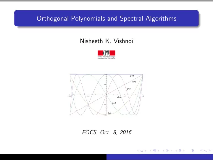
d=0 d=1 d=2 d=3 d=4 d=5

1.0 0.5 0.5 1.0 1.0 0.5 0.5 1.0

FOCS, Oct. 8, 2016

Orthogonal Polynomials

µ-orthogonality Polynomials p(x), q(x) are µ-orthogonal w.r.t. µ : I → R≥0 if p, qµ :=

• x∈I

p(x)q(x)dµ(x) = 0 µ-orthogonal family Start with 1, x, x2, . . . , xd, . . . and apply Gram-Schmidt

• rthogonalization w.r.t. ·, ·µ to obtain a µ-orthogonal family

p0(x) = 1, p1(x), p2(x), . . . , pd(x), . . . Examples Legendre: I = [−1, 1] and µ(x) = 1. Hermite: I = R and µ(x) = e−x2/2. Laguerre: I = R≥0 and µ(x) = e−x. Chebyshev (Type 1): I = [−1, 1] and µ(x) =

1 √ 1−x2 .

Orthogonal Polynomials

µ-orthogonality Polynomials p(x), q(x) are µ-orthogonal w.r.t. µ : I → R≥0 if p, qµ :=

• x∈I

p(x)q(x)dµ(x) = 0 µ-orthogonal family Start with 1, x, x2, . . . , xd, . . . and apply Gram-Schmidt

• rthogonalization w.r.t. ·, ·µ to obtain a µ-orthogonal family

p0(x) = 1, p1(x), p2(x), . . . , pd(x), . . . Examples Legendre: I = [−1, 1] and µ(x) = 1. Hermite: I = R and µ(x) = e−x2/2. Laguerre: I = R≥0 and µ(x) = e−x. Chebyshev (Type 1): I = [−1, 1] and µ(x) =

1 √ 1−x2 .

Orthogonal Polynomials

µ-orthogonality Polynomials p(x), q(x) are µ-orthogonal w.r.t. µ : I → R≥0 if p, qµ :=

• x∈I

p(x)q(x)dµ(x) = 0 µ-orthogonal family Start with 1, x, x2, . . . , xd, . . . and apply Gram-Schmidt

• rthogonalization w.r.t. ·, ·µ to obtain a µ-orthogonal family

p0(x) = 1, p1(x), p2(x), . . . , pd(x), . . . Examples Legendre: I = [−1, 1] and µ(x) = 1. Hermite: I = R and µ(x) = e−x2/2. Laguerre: I = R≥0 and µ(x) = e−x. Chebyshev (Type 1): I = [−1, 1] and µ(x) =

1 √ 1−x2 .

Orthgonal polynomials have many amazing properties

Monic µ-orthogonal polynomials satisfy 3-term recurrences pd+1(x) = (x − αd+1)pd + βdpd−1 for d ≥ 0 with p−1 = 0.

Orthgonal polynomials have many amazing properties

Monic µ-orthogonal polynomials satisfy 3-term recurrences pd+1(x) = (x − αd+1)pd + βdpd−1 for d ≥ 0 with p−1 = 0. Proof sketch

1

degree d

• pd+1 − xpd = αd+1pd + βdpd−1 +

i<d−1 γipi

Orthgonal polynomials have many amazing properties

Monic µ-orthogonal polynomials satisfy 3-term recurrences pd+1(x) = (x − αd+1)pd + βdpd−1 for d ≥ 0 with p−1 = 0. Proof sketch

1

degree d

• pd+1 − xpd = αd+1pd + βdpd−1 +

i<d−1 γipi

2 For i < d − 1, xpd, piµ = pd+1 − xpd, piµ = γipi, piµ but

Orthgonal polynomials have many amazing properties

Monic µ-orthogonal polynomials satisfy 3-term recurrences pd+1(x) = (x − αd+1)pd + βdpd−1 for d ≥ 0 with p−1 = 0. Proof sketch

1

degree d

• pd+1 − xpd = αd+1pd + βdpd−1 +

i<d−1 γipi

2 For i < d − 1, xpd, piµ = pd+1 − xpd, piµ = γipi, piµ but 3 xpd, piµ = pd, xpiµ = 0 as deg(xpi) < d implying γi = 0.

Orthgonal polynomials have many amazing properties

Monic µ-orthogonal polynomials satisfy 3-term recurrences pd+1(x) = (x − αd+1)pd + βdpd−1 for d ≥ 0 with p−1 = 0. Proof sketch

1

degree d

• pd+1 − xpd = αd+1pd + βdpd−1 +

i<d−1 γipi

2 For i < d − 1, xpd, piµ = pd+1 − xpd, piµ = γipi, piµ but 3 xpd, piµ = pd, xpiµ = 0 as deg(xpi) < d implying γi = 0.

Roots (corollaries) If p0, p1, . . . , pd, . . . are orthogonal w.r.t. µ : [a, b] → R≥0 then for each pd, roots are distinct, real and lie in [a, b]. Roots of pd and pd+1 also interlace!

Many and growing applications in TCS ...

Hermite: I = R and µ(x) = e−x2/2 Invariance principles, hardness of approximation a la Mossel, O’Donnell, Oleszkiewicz, ... Laguerre: I = R≥0 and µ(x) = e−x Constructing sparsifiers a la Batson, Marcus, Spielman, Srivastava, ... Chebyshev (Type 2): I = [−1, 1] and µ(x) = √ 1 − x2 Nonbacktracking random walks and Ramanujan graphs a la Alon, Boppana, Friedman, Lubotzky, Philips, Sarnak, ... Chebyshev (Type 1): I = [−1, 1] and µ(x) =

1 √ 1−x2

Spectral algorithms – This talk Extensions to multivariate and matrix polynomials Several examples in this workshop ..

Many and growing applications in TCS ...

Hermite: I = R and µ(x) = e−x2/2 Invariance principles, hardness of approximation a la Mossel, O’Donnell, Oleszkiewicz, ... Laguerre: I = R≥0 and µ(x) = e−x Constructing sparsifiers a la Batson, Marcus, Spielman, Srivastava, ... Chebyshev (Type 2): I = [−1, 1] and µ(x) = √ 1 − x2 Nonbacktracking random walks and Ramanujan graphs a la Alon, Boppana, Friedman, Lubotzky, Philips, Sarnak, ... Chebyshev (Type 1): I = [−1, 1] and µ(x) =

1 √ 1−x2

Spectral algorithms – This talk Extensions to multivariate and matrix polynomials Several examples in this workshop ..

Many and growing applications in TCS ...

Hermite: I = R and µ(x) = e−x2/2 Invariance principles, hardness of approximation a la Mossel, O’Donnell, Oleszkiewicz, ... Laguerre: I = R≥0 and µ(x) = e−x Constructing sparsifiers a la Batson, Marcus, Spielman, Srivastava, ... Chebyshev (Type 2): I = [−1, 1] and µ(x) = √ 1 − x2 Nonbacktracking random walks and Ramanujan graphs a la Alon, Boppana, Friedman, Lubotzky, Philips, Sarnak, ... Chebyshev (Type 1): I = [−1, 1] and µ(x) =

1 √ 1−x2

Spectral algorithms – This talk Extensions to multivariate and matrix polynomials Several examples in this workshop ..

Many and growing applications in TCS ...

Hermite: I = R and µ(x) = e−x2/2 Invariance principles, hardness of approximation a la Mossel, O’Donnell, Oleszkiewicz, ... Laguerre: I = R≥0 and µ(x) = e−x Constructing sparsifiers a la Batson, Marcus, Spielman, Srivastava, ... Chebyshev (Type 2): I = [−1, 1] and µ(x) = √ 1 − x2 Nonbacktracking random walks and Ramanujan graphs a la Alon, Boppana, Friedman, Lubotzky, Philips, Sarnak, ... Chebyshev (Type 1): I = [−1, 1] and µ(x) =

1 √ 1−x2

Spectral algorithms – This talk Extensions to multivariate and matrix polynomials Several examples in this workshop ..

Many and growing applications in TCS ...

Hermite: I = R and µ(x) = e−x2/2 Invariance principles, hardness of approximation a la Mossel, O’Donnell, Oleszkiewicz, ... Laguerre: I = R≥0 and µ(x) = e−x Constructing sparsifiers a la Batson, Marcus, Spielman, Srivastava, ... Chebyshev (Type 2): I = [−1, 1] and µ(x) = √ 1 − x2 Nonbacktracking random walks and Ramanujan graphs a la Alon, Boppana, Friedman, Lubotzky, Philips, Sarnak, ... Chebyshev (Type 1): I = [−1, 1] and µ(x) =

1 √ 1−x2

Spectral algorithms – This talk Extensions to multivariate and matrix polynomials Several examples in this workshop ..

The goal of today’s talk

Many spectral algorithms today rely on ability to quickly compute good approximations to matrix-function-vector products: e.g., Asv, A−1v, exp(−A)v, ...

• r top few eigenvalues and eigenvectors.

Demonstrate How to reduce the problem of computing these primitives to a small number of computations of the form Bu where B is a matrix closely related to A (often A itself) and u is some vector. A key feature: If Av can be computed quickly (e.g., if A is sparse) then Bu can also be computed quickly. Approximation theory provides the right framework to study these questions – Borrows heavily from orthogonal polynomials!

The goal of today’s talk

Many spectral algorithms today rely on ability to quickly compute good approximations to matrix-function-vector products: e.g., Asv, A−1v, exp(−A)v, ...

• r top few eigenvalues and eigenvectors.

Demonstrate How to reduce the problem of computing these primitives to a small number of computations of the form Bu where B is a matrix closely related to A (often A itself) and u is some vector. A key feature: If Av can be computed quickly (e.g., if A is sparse) then Bu can also be computed quickly. Approximation theory provides the right framework to study these questions – Borrows heavily from orthogonal polynomials!

The goal of today’s talk

Many spectral algorithms today rely on ability to quickly compute good approximations to matrix-function-vector products: e.g., Asv, A−1v, exp(−A)v, ...

• r top few eigenvalues and eigenvectors.

Demonstrate How to reduce the problem of computing these primitives to a small number of computations of the form Bu where B is a matrix closely related to A (often A itself) and u is some vector. A key feature: If Av can be computed quickly (e.g., if A is sparse) then Bu can also be computed quickly. Approximation theory provides the right framework to study these questions – Borrows heavily from orthogonal polynomials!

The goal of today’s talk

Many spectral algorithms today rely on ability to quickly compute good approximations to matrix-function-vector products: e.g., Asv, A−1v, exp(−A)v, ...

• r top few eigenvalues and eigenvectors.

Demonstrate How to reduce the problem of computing these primitives to a small number of computations of the form Bu where B is a matrix closely related to A (often A itself) and u is some vector. A key feature: If Av can be computed quickly (e.g., if A is sparse) then Bu can also be computed quickly. Approximation theory provides the right framework to study these questions – Borrows heavily from orthogonal polynomials!

The goal of today’s talk

Many spectral algorithms today rely on ability to quickly compute good approximations to matrix-function-vector products: e.g., Asv, A−1v, exp(−A)v, ...

• r top few eigenvalues and eigenvectors.

Demonstrate How to reduce the problem of computing these primitives to a small number of computations of the form Bu where B is a matrix closely related to A (often A itself) and u is some vector. A key feature: If Av can be computed quickly (e.g., if A is sparse) then Bu can also be computed quickly. Approximation theory provides the right framework to study these questions – Borrows heavily from orthogonal polynomials!

Approximation Theory

Approximation Theory

Approximation Theory

Approximation Theory

Approximation Theory

How well can functions be approximated by simpler ones? Uniform (Chebyshev) Approximation by Polynomials/Rationals For f : R → R and an interval I, what is the closest a degree d polynomial/rational function can remain to f (x) throughout I inf

p∈Σd

sup

x∈I

|f (x) − p(x)|. inf

p,q∈Σd

sup

x∈I

|f (x) − p(x)/q(x)|.

Σd: set of all polynomials of degree at most d.

150+ years of fascinating history, deep results and many applications. Interested in fundamental functions such as xs, e−x and 1/x

• ver finite and infinite intervals such as [−1, 1], [0, n], [0, ∞).

For our applications good enough approximations suffice.

Approximation Theory

How well can functions be approximated by simpler ones? Uniform (Chebyshev) Approximation by Polynomials/Rationals For f : R → R and an interval I, what is the closest a degree d polynomial/rational function can remain to f (x) throughout I inf

p∈Σd

sup

x∈I

|f (x) − p(x)|. inf

p,q∈Σd

sup

x∈I

|f (x) − p(x)/q(x)|.

Σd: set of all polynomials of degree at most d.

150+ years of fascinating history, deep results and many applications. Interested in fundamental functions such as xs, e−x and 1/x

• ver finite and infinite intervals such as [−1, 1], [0, n], [0, ∞).

For our applications good enough approximations suffice.

Approximation Theory

How well can functions be approximated by simpler ones? Uniform (Chebyshev) Approximation by Polynomials/Rationals For f : R → R and an interval I, what is the closest a degree d polynomial/rational function can remain to f (x) throughout I inf

p∈Σd

sup

x∈I

|f (x) − p(x)|. inf

p,q∈Σd

sup

x∈I

|f (x) − p(x)/q(x)|.

Σd: set of all polynomials of degree at most d.

150+ years of fascinating history, deep results and many applications. Interested in fundamental functions such as xs, e−x and 1/x

• ver finite and infinite intervals such as [−1, 1], [0, n], [0, ∞).

For our applications good enough approximations suffice.

Approximation Theory

How well can functions be approximated by simpler ones? Uniform (Chebyshev) Approximation by Polynomials/Rationals For f : R → R and an interval I, what is the closest a degree d polynomial/rational function can remain to f (x) throughout I inf

p∈Σd

sup

x∈I

|f (x) − p(x)|. inf

p,q∈Σd

sup

x∈I

|f (x) − p(x)/q(x)|.

Σd: set of all polynomials of degree at most d.

150+ years of fascinating history, deep results and many applications. Interested in fundamental functions such as xs, e−x and 1/x

• ver finite and infinite intervals such as [−1, 1], [0, n], [0, ∞).

For our applications good enough approximations suffice.

Approximation Theory

How well can functions be approximated by simpler ones? Uniform (Chebyshev) Approximation by Polynomials/Rationals For f : R → R and an interval I, what is the closest a degree d polynomial/rational function can remain to f (x) throughout I inf

p∈Σd

sup

x∈I

|f (x) − p(x)|. inf

p,q∈Σd

sup

x∈I

|f (x) − p(x)/q(x)|.

Σd: set of all polynomials of degree at most d.

150+ years of fascinating history, deep results and many applications. Interested in fundamental functions such as xs, e−x and 1/x

• ver finite and infinite intervals such as [−1, 1], [0, n], [0, ∞).

For our applications good enough approximations suffice.

Approximation Theory

How well can functions be approximated by simpler ones? Uniform (Chebyshev) Approximation by Polynomials/Rationals For f : R → R and an interval I, what is the closest a degree d polynomial/rational function can remain to f (x) throughout I inf

p∈Σd

sup

x∈I

|f (x) − p(x)|. inf

p,q∈Σd

sup

x∈I

|f (x) − p(x)/q(x)|.

Σd: set of all polynomials of degree at most d.

150+ years of fascinating history, deep results and many applications. Interested in fundamental functions such as xs, e−x and 1/x

• ver finite and infinite intervals such as [−1, 1], [0, n], [0, ∞).

For our applications good enough approximations suffice.

Algorithms/Numerical Linear Alg.- f (A)v, Eigenvalues, ..

A simple example: Compute Asv where A is symmetric with eigenvalues in [−1, 1], v is a vector and s is a large positive integer. The straightforward way to compute Asv takes time O(ms) where m is the number of non-zero entries in A. Suppose xs can be δ-approximated over the interval [−1, 1] by a degree d polynomial ps,d(x) = d

i=0 aixi.

Candidate approximation to Asv: d

i=0 aiAiv.

The time to compute d

i=0 aiAiv is O(md).

d

i=0 aiAiv − Asv ≤ δv since

all the eigenvalues of A lie in [−1, 1], and ps,d is δ-close to xs in the entire interval [−1, 1].

How small can d be?

Algorithms/Numerical Linear Alg.- f (A)v, Eigenvalues, ..

A simple example: Compute Asv where A is symmetric with eigenvalues in [−1, 1], v is a vector and s is a large positive integer. The straightforward way to compute Asv takes time O(ms) where m is the number of non-zero entries in A. Suppose xs can be δ-approximated over the interval [−1, 1] by a degree d polynomial ps,d(x) = d

i=0 aixi.

Candidate approximation to Asv: d

i=0 aiAiv.

The time to compute d

i=0 aiAiv is O(md).

d

i=0 aiAiv − Asv ≤ δv since

all the eigenvalues of A lie in [−1, 1], and ps,d is δ-close to xs in the entire interval [−1, 1].

How small can d be?

Algorithms/Numerical Linear Alg.- f (A)v, Eigenvalues, ..

A simple example: Compute Asv where A is symmetric with eigenvalues in [−1, 1], v is a vector and s is a large positive integer. The straightforward way to compute Asv takes time O(ms) where m is the number of non-zero entries in A. Suppose xs can be δ-approximated over the interval [−1, 1] by a degree d polynomial ps,d(x) = d

i=0 aixi.

Candidate approximation to Asv: d

i=0 aiAiv.

The time to compute d

i=0 aiAiv is O(md).

d

i=0 aiAiv − Asv ≤ δv since

all the eigenvalues of A lie in [−1, 1], and ps,d is δ-close to xs in the entire interval [−1, 1].

How small can d be?

Algorithms/Numerical Linear Alg.- f (A)v, Eigenvalues, ..

A simple example: Compute Asv where A is symmetric with eigenvalues in [−1, 1], v is a vector and s is a large positive integer. The straightforward way to compute Asv takes time O(ms) where m is the number of non-zero entries in A. Suppose xs can be δ-approximated over the interval [−1, 1] by a degree d polynomial ps,d(x) = d

i=0 aixi.

Candidate approximation to Asv: d

i=0 aiAiv.

The time to compute d

i=0 aiAiv is O(md).

d

i=0 aiAiv − Asv ≤ δv since

all the eigenvalues of A lie in [−1, 1], and ps,d is δ-close to xs in the entire interval [−1, 1].

How small can d be?

Algorithms/Numerical Linear Alg.- f (A)v, Eigenvalues, ..

A simple example: Compute Asv where A is symmetric with eigenvalues in [−1, 1], v is a vector and s is a large positive integer. The straightforward way to compute Asv takes time O(ms) where m is the number of non-zero entries in A. Suppose xs can be δ-approximated over the interval [−1, 1] by a degree d polynomial ps,d(x) = d

i=0 aixi.

Candidate approximation to Asv: d

i=0 aiAiv.

The time to compute d

i=0 aiAiv is O(md).

d

i=0 aiAiv − Asv ≤ δv since

all the eigenvalues of A lie in [−1, 1], and ps,d is δ-close to xs in the entire interval [−1, 1].

How small can d be?

Algorithms/Numerical Linear Alg.- f (A)v, Eigenvalues, ..

A simple example: Compute Asv where A is symmetric with eigenvalues in [−1, 1], v is a vector and s is a large positive integer. The straightforward way to compute Asv takes time O(ms) where m is the number of non-zero entries in A. Suppose xs can be δ-approximated over the interval [−1, 1] by a degree d polynomial ps,d(x) = d

i=0 aixi.

Candidate approximation to Asv: d

i=0 aiAiv.

The time to compute d

i=0 aiAiv is O(md).

d

i=0 aiAiv − Asv ≤ δv since

all the eigenvalues of A lie in [−1, 1], and ps,d is δ-close to xs in the entire interval [−1, 1].

How small can d be?

Algorithms/Numerical Linear Alg.- f (A)v, Eigenvalues, ..

A simple example: Compute Asv where A is symmetric with eigenvalues in [−1, 1], v is a vector and s is a large positive integer. The straightforward way to compute Asv takes time O(ms) where m is the number of non-zero entries in A. Suppose xs can be δ-approximated over the interval [−1, 1] by a degree d polynomial ps,d(x) = d

i=0 aixi.

Candidate approximation to Asv: d

i=0 aiAiv.

The time to compute d

i=0 aiAiv is O(md).

d

i=0 aiAiv − Asv ≤ δv since

all the eigenvalues of A lie in [−1, 1], and ps,d is δ-close to xs in the entire interval [−1, 1].

How small can d be?

Algorithms/Numerical Linear Alg.- f (A)v, Eigenvalues, ..

A simple example: Compute Asv where A is symmetric with eigenvalues in [−1, 1], v is a vector and s is a large positive integer. The straightforward way to compute Asv takes time O(ms) where m is the number of non-zero entries in A. Suppose xs can be δ-approximated over the interval [−1, 1] by a degree d polynomial ps,d(x) = d

i=0 aixi.

Candidate approximation to Asv: d

i=0 aiAiv.

The time to compute d

i=0 aiAiv is O(md).

d

i=0 aiAiv − Asv ≤ δv since

all the eigenvalues of A lie in [−1, 1], and ps,d is δ-close to xs in the entire interval [−1, 1].

How small can d be?

Example: Approximating the Monomial

For any s, for any δ > 0, and d ∼

• s log (1/δ), there is a

polynomial ps,d s.t. sup

x∈[−1,1]

|ps,d(x) − xs| ≤ δ. Simulating Random Walks: If A is random walk matrix of a graph, we can simulate s steps of a random walk in m√s time. Conjugate Gradient Method: Given Ax = b with eigenvalues of A in (0, 1], one can find y s.t. y − A−1bA ≤ δA−1bA in time roughly m

• κ(A) log 1/δ.

Quadratic speedup over the Power Method: Given A, in time ∼ m/

√ δ can compute a value µ ∈ [(1 − δ)λ1(A), λ1(A)].

Example: Approximating the Monomial

For any s, for any δ > 0, and d ∼

• s log (1/δ), there is a

polynomial ps,d s.t. sup

x∈[−1,1]

|ps,d(x) − xs| ≤ δ. Simulating Random Walks: If A is random walk matrix of a graph, we can simulate s steps of a random walk in m√s time. Conjugate Gradient Method: Given Ax = b with eigenvalues of A in (0, 1], one can find y s.t. y − A−1bA ≤ δA−1bA in time roughly m

• κ(A) log 1/δ.

Quadratic speedup over the Power Method: Given A, in time ∼ m/

√ δ can compute a value µ ∈ [(1 − δ)λ1(A), λ1(A)].

Example: Approximating the Monomial

For any s, for any δ > 0, and d ∼

• s log (1/δ), there is a

polynomial ps,d s.t. sup

x∈[−1,1]

|ps,d(x) − xs| ≤ δ. Simulating Random Walks: If A is random walk matrix of a graph, we can simulate s steps of a random walk in m√s time. Conjugate Gradient Method: Given Ax = b with eigenvalues of A in (0, 1], one can find y s.t. y − A−1bA ≤ δA−1bA in time roughly m

• κ(A) log 1/δ.

Quadratic speedup over the Power Method: Given A, in time ∼ m/

√ δ can compute a value µ ∈ [(1 − δ)λ1(A), λ1(A)].

Example: Approximating the Monomial

For any s, for any δ > 0, and d ∼

• s log (1/δ), there is a

polynomial ps,d s.t. sup

x∈[−1,1]

|ps,d(x) − xs| ≤ δ. Simulating Random Walks: If A is random walk matrix of a graph, we can simulate s steps of a random walk in m√s time. Conjugate Gradient Method: Given Ax = b with eigenvalues of A in (0, 1], one can find y s.t. y − A−1bA ≤ δA−1bA in time roughly m

• κ(A) log 1/δ.

Quadratic speedup over the Power Method: Given A, in time ∼ m/

√ δ can compute a value µ ∈ [(1 − δ)λ1(A), λ1(A)].

Chebyshev Polynomials

Recall: Chebyshev polynomial orthogonal w.r.t.

1 √ 1−x2 over [−1, 1]

Td+1(x) = 2xTd(x) − Td−1(x) Averaging Property xTd(x) = Td+1(x)+Td−1(x)

2

. Boundedness Property For any θ, and any integer d, Td(cos θ) = cos(dθ). Thus, |Td(x)| ≤ 1 for all x ∈ [−1, 1].

Chebyshev Polynomials

Recall: Chebyshev polynomial orthogonal w.r.t.

1 √ 1−x2 over [−1, 1]

Td+1(x) = 2xTd(x) − Td−1(x) Averaging Property xTd(x) = Td+1(x)+Td−1(x)

2

. Boundedness Property For any θ, and any integer d, Td(cos θ) = cos(dθ). Thus, |Td(x)| ≤ 1 for all x ∈ [−1, 1].

Chebyshev Polynomials

Recall: Chebyshev polynomial orthogonal w.r.t.

1 √ 1−x2 over [−1, 1]

Td+1(x) = 2xTd(x) − Td−1(x) Averaging Property xTd(x) = Td+1(x)+Td−1(x)

2

. Boundedness Property For any θ, and any integer d, Td(cos θ) = cos(dθ). Thus, |Td(x)| ≤ 1 for all x ∈ [−1, 1].

Chebyshev Polynomials

Recall: Chebyshev polynomial orthogonal w.r.t.

1 √ 1−x2 over [−1, 1]

Td+1(x) = 2xTd(x) − Td−1(x) Averaging Property xTd(x) = Td+1(x)+Td−1(x)

2

. Boundedness Property For any θ, and any integer d, Td(cos θ) = cos(dθ). Thus, |Td(x)| ≤ 1 for all x ∈ [−1, 1].

Back to Approximating Monomials

Ds

def

= s

i=1 Yi where Y1, . . . , Ys i.i.d. ±1 w.p. 1/2 (D0 def

= 0). Thus, Pr

• |Ds| ≥
• 2s log (2/δ)
• ≤ δ.

Key Claim: E

Y1,...,Ys[TDs(x)] = xs.

xs+1 = x · E

Y1,...,Ys TDs(x) =

E

Y1,...,Ys[x · TDs(x)]

= E

Y1,...,Ys [1/2(TDs+1(x) + TDs−1(x))] =

E

Y1,...,Ys+1[TDs+1(x)].

Our Approximation to xs: ps,d(x) def = E

Y1,...,Ys

• TDs(x) · 1|Ds|≤d
• for d =
• 2s log (2/δ).

sup

x∈[−1,1]

|ps,d(x) − xs| = sup

x∈[−1,1]

• E

Y1,...,Ys

• TDs(x) · 1|Ds|>d
• ≤

E

Y1,...,Ys

• 1|Ds|>d ·

sup

x∈[−1,1]

|TDs(x)|

• ≤

E

Y1,...,Ys

• 1|Ds|>d
• ≤ δ.

Back to Approximating Monomials

Ds

def

= s

i=1 Yi where Y1, . . . , Ys i.i.d. ±1 w.p. 1/2 (D0 def

= 0). Thus, Pr

• |Ds| ≥
• 2s log (2/δ)
• ≤ δ.

Key Claim: E

Y1,...,Ys[TDs(x)] = xs.

xs+1 = x · E

Y1,...,Ys TDs(x) =

E

Y1,...,Ys[x · TDs(x)]

= E

Y1,...,Ys [1/2(TDs+1(x) + TDs−1(x))] =

E

Y1,...,Ys+1[TDs+1(x)].

Our Approximation to xs: ps,d(x) def = E

Y1,...,Ys

• TDs(x) · 1|Ds|≤d
• for d =
• 2s log (2/δ).

sup

x∈[−1,1]

|ps,d(x) − xs| = sup

x∈[−1,1]

• E

Y1,...,Ys

• TDs(x) · 1|Ds|>d
• ≤

E

Y1,...,Ys

• 1|Ds|>d ·

sup

x∈[−1,1]

|TDs(x)|

• ≤

E

Y1,...,Ys

• 1|Ds|>d
• ≤ δ.

Back to Approximating Monomials

Ds

def

= s

i=1 Yi where Y1, . . . , Ys i.i.d. ±1 w.p. 1/2 (D0 def

= 0). Thus, Pr

• |Ds| ≥
• 2s log (2/δ)
• ≤ δ.

Key Claim: E

Y1,...,Ys[TDs(x)] = xs.

xs+1 = x · E

Y1,...,Ys TDs(x) =

E

Y1,...,Ys[x · TDs(x)]

= E

Y1,...,Ys [1/2(TDs+1(x) + TDs−1(x))] =

E

Y1,...,Ys+1[TDs+1(x)].

Our Approximation to xs: ps,d(x) def = E

Y1,...,Ys

• TDs(x) · 1|Ds|≤d
• for d =
• 2s log (2/δ).

sup

x∈[−1,1]

|ps,d(x) − xs| = sup

x∈[−1,1]

• E

Y1,...,Ys

• TDs(x) · 1|Ds|>d
• ≤

E

Y1,...,Ys

• 1|Ds|>d ·

sup

x∈[−1,1]

|TDs(x)|

• ≤

E

Y1,...,Ys

• 1|Ds|>d
• ≤ δ.

Back to Approximating Monomials

Ds

def

= s

i=1 Yi where Y1, . . . , Ys i.i.d. ±1 w.p. 1/2 (D0 def

= 0). Thus, Pr

• |Ds| ≥
• 2s log (2/δ)
• ≤ δ.

Key Claim: E

Y1,...,Ys[TDs(x)] = xs.

xs+1 = x · E

Y1,...,Ys TDs(x) =

E

Y1,...,Ys[x · TDs(x)]

= E

Y1,...,Ys [1/2(TDs+1(x) + TDs−1(x))] =

E

Y1,...,Ys+1[TDs+1(x)].

Our Approximation to xs: ps,d(x) def = E

Y1,...,Ys

• TDs(x) · 1|Ds|≤d
• for d =
• 2s log (2/δ).

sup

x∈[−1,1]

|ps,d(x) − xs| = sup

x∈[−1,1]

• E

Y1,...,Ys

• TDs(x) · 1|Ds|>d
• ≤

E

Y1,...,Ys

• 1|Ds|>d ·

sup

x∈[−1,1]

|TDs(x)|

• ≤

E

Y1,...,Ys

• 1|Ds|>d
• ≤ δ.

Back to Approximating Monomials

Ds

def

= s

i=1 Yi where Y1, . . . , Ys i.i.d. ±1 w.p. 1/2 (D0 def

= 0). Thus, Pr

• |Ds| ≥
• 2s log (2/δ)
• ≤ δ.

Key Claim: E

Y1,...,Ys[TDs(x)] = xs.

xs+1 = x · E

Y1,...,Ys TDs(x) =

E

Y1,...,Ys[x · TDs(x)]

= E

Y1,...,Ys [1/2(TDs+1(x) + TDs−1(x))] =

E

Y1,...,Ys+1[TDs+1(x)].

Our Approximation to xs: ps,d(x) def = E

Y1,...,Ys

• TDs(x) · 1|Ds|≤d
• for d =
• 2s log (2/δ).

sup

x∈[−1,1]

|ps,d(x) − xs| = sup

x∈[−1,1]

• E

Y1,...,Ys

• TDs(x) · 1|Ds|>d
• ≤

E

Y1,...,Ys

• 1|Ds|>d ·

sup

x∈[−1,1]

|TDs(x)|

• ≤

E

Y1,...,Ys

• 1|Ds|>d
• ≤ δ.

Back to Approximating Monomials

Ds

def

= s

i=1 Yi where Y1, . . . , Ys i.i.d. ±1 w.p. 1/2 (D0 def

= 0). Thus, Pr

• |Ds| ≥
• 2s log (2/δ)
• ≤ δ.

Key Claim: E

Y1,...,Ys[TDs(x)] = xs.

xs+1 = x · E

Y1,...,Ys TDs(x) =

E

Y1,...,Ys[x · TDs(x)]

= E

Y1,...,Ys [1/2(TDs+1(x) + TDs−1(x))] =

E

Y1,...,Ys+1[TDs+1(x)].

Our Approximation to xs: ps,d(x) def = E

Y1,...,Ys

• TDs(x) · 1|Ds|≤d
• for d =
• 2s log (2/δ).

sup

x∈[−1,1]

|ps,d(x) − xs| = sup

x∈[−1,1]

• E

Y1,...,Ys

• TDs(x) · 1|Ds|>d
• ≤

E

Y1,...,Ys

• 1|Ds|>d ·

sup

x∈[−1,1]

|TDs(x)|

• ≤

E

Y1,...,Ys

• 1|Ds|>d
• ≤ δ.

A General Recipe?

Let f (x) be δ-approximated by a Taylor polynomial k

s=0 csxs.

Then, one may instead try the approx. (with suitably shifted ps,d)

k

• s=0

csps,√

s log 1/δ(x)

. Approximating the Exponential For every b > 0, and δ, there is a polynomial rb,δ s.t. supx∈[0,b] |e−x − rb,δ(x)| ≤ δ; degree ∼

• b log 1/δ. (Taylor -Ω(b).)

Implies ˜ O(m

• A log 1/δ) time algorithm to compute a

δ-approximation to e−Av for a PSD A. Useful in solving SDPs. When A is a graph Laplacian, implies an optimal spectral algorithm for Balanced Separator that runs in time ˜ O(m/√γ). (γ is the target conductance) [Orecchia-Sachdeva-V. 2012].

How far can polynomial approximations take us?

A General Recipe?

Let f (x) be δ-approximated by a Taylor polynomial k

s=0 csxs.

Then, one may instead try the approx. (with suitably shifted ps,d)

k

• s=0

csps,√

s log 1/δ(x)

. Approximating the Exponential For every b > 0, and δ, there is a polynomial rb,δ s.t. supx∈[0,b] |e−x − rb,δ(x)| ≤ δ; degree ∼

• b log 1/δ. (Taylor -Ω(b).)

Implies ˜ O(m

• A log 1/δ) time algorithm to compute a

δ-approximation to e−Av for a PSD A. Useful in solving SDPs. When A is a graph Laplacian, implies an optimal spectral algorithm for Balanced Separator that runs in time ˜ O(m/√γ). (γ is the target conductance) [Orecchia-Sachdeva-V. 2012].

How far can polynomial approximations take us?

A General Recipe?

Let f (x) be δ-approximated by a Taylor polynomial k

s=0 csxs.

Then, one may instead try the approx. (with suitably shifted ps,d)

k

• s=0

csps,√

s log 1/δ(x)

. Approximating the Exponential For every b > 0, and δ, there is a polynomial rb,δ s.t. supx∈[0,b] |e−x − rb,δ(x)| ≤ δ; degree ∼

• b log 1/δ. (Taylor -Ω(b).)

Implies ˜ O(m

• A log 1/δ) time algorithm to compute a

δ-approximation to e−Av for a PSD A. Useful in solving SDPs. When A is a graph Laplacian, implies an optimal spectral algorithm for Balanced Separator that runs in time ˜ O(m/√γ). (γ is the target conductance) [Orecchia-Sachdeva-V. 2012].

How far can polynomial approximations take us?

A General Recipe?

Let f (x) be δ-approximated by a Taylor polynomial k

s=0 csxs.

Then, one may instead try the approx. (with suitably shifted ps,d)

k

• s=0

csps,√

s log 1/δ(x)

. Approximating the Exponential For every b > 0, and δ, there is a polynomial rb,δ s.t. supx∈[0,b] |e−x − rb,δ(x)| ≤ δ; degree ∼

• b log 1/δ. (Taylor -Ω(b).)

Implies ˜ O(m

• A log 1/δ) time algorithm to compute a

δ-approximation to e−Av for a PSD A. Useful in solving SDPs. When A is a graph Laplacian, implies an optimal spectral algorithm for Balanced Separator that runs in time ˜ O(m/√γ). (γ is the target conductance) [Orecchia-Sachdeva-V. 2012].

How far can polynomial approximations take us?

A General Recipe?

Let f (x) be δ-approximated by a Taylor polynomial k

s=0 csxs.

Then, one may instead try the approx. (with suitably shifted ps,d)

k

• s=0

csps,√

s log 1/δ(x)

. Approximating the Exponential For every b > 0, and δ, there is a polynomial rb,δ s.t. supx∈[0,b] |e−x − rb,δ(x)| ≤ δ; degree ∼

• b log 1/δ. (Taylor -Ω(b).)

Implies ˜ O(m

• A log 1/δ) time algorithm to compute a

δ-approximation to e−Av for a PSD A. Useful in solving SDPs. When A is a graph Laplacian, implies an optimal spectral algorithm for Balanced Separator that runs in time ˜ O(m/√γ). (γ is the target conductance) [Orecchia-Sachdeva-V. 2012].

How far can polynomial approximations take us?

Lower Bounds for Polynomial Approximations

Bad News [see Sachdeva-V. 2014] Polynomial approx. to xs on [−1, 1] requires degree Ω(√s). Polynomial approx. to e−x on [0, b] requires degree Ω( √ b). Markov’s Theorem (inspired by a prob. of Mendeleev in Chemistry) Any degree-d polynomial p s.t. |p(x)| ≤ 1 over [−1, 1] must have its derivative |p(1)(x)| ≤ d2 for all x ∈ [−1, 1].

Chebyshev polynomials are a tight example for this theorem.

Bypass this barrier via rational functions!

Lower Bounds for Polynomial Approximations

Bad News [see Sachdeva-V. 2014] Polynomial approx. to xs on [−1, 1] requires degree Ω(√s). Polynomial approx. to e−x on [0, b] requires degree Ω( √ b). Markov’s Theorem (inspired by a prob. of Mendeleev in Chemistry) Any degree-d polynomial p s.t. |p(x)| ≤ 1 over [−1, 1] must have its derivative |p(1)(x)| ≤ d2 for all x ∈ [−1, 1].

Chebyshev polynomials are a tight example for this theorem.

Bypass this barrier via rational functions!

Lower Bounds for Polynomial Approximations

Bad News [see Sachdeva-V. 2014] Polynomial approx. to xs on [−1, 1] requires degree Ω(√s). Polynomial approx. to e−x on [0, b] requires degree Ω( √ b). Markov’s Theorem (inspired by a prob. of Mendeleev in Chemistry) Any degree-d polynomial p s.t. |p(x)| ≤ 1 over [−1, 1] must have its derivative |p(1)(x)| ≤ d2 for all x ∈ [−1, 1].

Chebyshev polynomials are a tight example for this theorem.

Bypass this barrier via rational functions!

Lower Bounds for Polynomial Approximations

Bad News [see Sachdeva-V. 2014] Polynomial approx. to xs on [−1, 1] requires degree Ω(√s). Polynomial approx. to e−x on [0, b] requires degree Ω( √ b). Markov’s Theorem (inspired by a prob. of Mendeleev in Chemistry) Any degree-d polynomial p s.t. |p(x)| ≤ 1 over [−1, 1] must have its derivative |p(1)(x)| ≤ d2 for all x ∈ [−1, 1].

Chebyshev polynomials are a tight example for this theorem.

Bypass this barrier via rational functions!

Example: Approximating the Exponential

For all integers d ≥ 0, there is a degree-d polynomial Sd(x) s.t. supx∈[0,∞)

• e−x −

1 Sd(x)

• ≤ 2−Ω(d).

Sd(x) def = d

k=0 xk k! . (Proof by induction.)

No dependence on the length of the interval! Hence, for any δ > 0, we have a rational function of degree O(log 1/δ) that is a δ-approximation to e−x. For most applications, an error of δ = 1/poly(n) suffices, so we can choose d = O(log n). Thus, (Sd(A))−1 v δ-approximates e−Av.

How do we compute (Sd(A))−1 v?

Example: Approximating the Exponential

For all integers d ≥ 0, there is a degree-d polynomial Sd(x) s.t. supx∈[0,∞)

• e−x −

1 Sd(x)

• ≤ 2−Ω(d).

Sd(x) def = d

k=0 xk k! . (Proof by induction.)

No dependence on the length of the interval! Hence, for any δ > 0, we have a rational function of degree O(log 1/δ) that is a δ-approximation to e−x. For most applications, an error of δ = 1/poly(n) suffices, so we can choose d = O(log n). Thus, (Sd(A))−1 v δ-approximates e−Av.

How do we compute (Sd(A))−1 v?

Example: Approximating the Exponential

For all integers d ≥ 0, there is a degree-d polynomial Sd(x) s.t. supx∈[0,∞)

• e−x −

1 Sd(x)

• ≤ 2−Ω(d).

Sd(x) def = d

k=0 xk k! . (Proof by induction.)

No dependence on the length of the interval! Hence, for any δ > 0, we have a rational function of degree O(log 1/δ) that is a δ-approximation to e−x. For most applications, an error of δ = 1/poly(n) suffices, so we can choose d = O(log n). Thus, (Sd(A))−1 v δ-approximates e−Av.

How do we compute (Sd(A))−1 v?

Example: Approximating the Exponential

For all integers d ≥ 0, there is a degree-d polynomial Sd(x) s.t. supx∈[0,∞)

• e−x −

1 Sd(x)

• ≤ 2−Ω(d).

Sd(x) def = d

k=0 xk k! . (Proof by induction.)

No dependence on the length of the interval! Hence, for any δ > 0, we have a rational function of degree O(log 1/δ) that is a δ-approximation to e−x. For most applications, an error of δ = 1/poly(n) suffices, so we can choose d = O(log n). Thus, (Sd(A))−1 v δ-approximates e−Av.

How do we compute (Sd(A))−1 v?

Example: Approximating the Exponential

For all integers d ≥ 0, there is a degree-d polynomial Sd(x) s.t. supx∈[0,∞)

• e−x −

1 Sd(x)

• ≤ 2−Ω(d).

Sd(x) def = d

k=0 xk k! . (Proof by induction.)

No dependence on the length of the interval! Hence, for any δ > 0, we have a rational function of degree O(log 1/δ) that is a δ-approximation to e−x. For most applications, an error of δ = 1/poly(n) suffices, so we can choose d = O(log n). Thus, (Sd(A))−1 v δ-approximates e−Av.

How do we compute (Sd(A))−1 v?

Example: Approximating the Exponential

For all integers d ≥ 0, there is a degree-d polynomial Sd(x) s.t. supx∈[0,∞)

• e−x −

1 Sd(x)

• ≤ 2−Ω(d).

Sd(x) def = d

k=0 xk k! . (Proof by induction.)

No dependence on the length of the interval! Hence, for any δ > 0, we have a rational function of degree O(log 1/δ) that is a δ-approximation to e−x. For most applications, an error of δ = 1/poly(n) suffices, so we can choose d = O(log n). Thus, (Sd(A))−1 v δ-approximates e−Av.

How do we compute (Sd(A))−1 v?

Rational Approximations with Negative Poles

Factor Sd(x) = α0 d

i=1(x − βi) and output α0

d

i=1(A − βiI)−1v.

Rational Approximations with Negative Poles

Factor Sd(x) = α0 d

i=1(x − βi) and output α0

d

i=1(A − βiI)−1v.

Since d is O(log n), it suffices to compute (A − βiI)−1u.

Rational Approximations with Negative Poles

Factor Sd(x) = α0 d

i=1(x − βi) and output α0

d

i=1(A − βiI)−1v.

Since d is O(log n), it suffices to compute (A − βiI)−1u. When A is Laplacian, and βi ≤ 0, then A − βiI is SDD!

Rational Approximations with Negative Poles

Factor Sd(x) = α0 d

i=1(x − βi) and output α0

d

i=1(A − βiI)−1v.

Since d is O(log n), it suffices to compute (A − βiI)−1u. When A is Laplacian, and βi ≤ 0, then A − βiI is SDD! Saff-Sch¨

• nhage-Varga 1975

For every d, there exists a degree-d polynomial pd s.t., sup

x∈[0,∞)

• e−x − pd
• 1

1+x/d

• ≤ 2−Ω(d).

Rational Approximations with Negative Poles

Factor Sd(x) = α0 d

i=1(x − βi) and output α0

d

i=1(A − βiI)−1v.

Since d is O(log n), it suffices to compute (A − βiI)−1u. When A is Laplacian, and βi ≤ 0, then A − βiI is SDD! Saff-Sch¨

• nhage-Varga 1975

For every d, there exists a degree-d polynomial pd s.t., sup

x∈[0,∞)

• e−x − pd
• 1

1+x/d

• ≤ 2−Ω(d).

Proof uses properties of Legendre, Laguerre polynomials!

Rational Approximations with Negative Poles

Factor Sd(x) = α0 d

i=1(x − βi) and output α0

d

i=1(A − βiI)−1v.

Since d is O(log n), it suffices to compute (A − βiI)−1u. When A is Laplacian, and βi ≤ 0, then A − βiI is SDD! Saff-Sch¨

• nhage-Varga 1975

For every d, there exists a degree-d polynomial pd s.t., sup

x∈[0,∞)

• e−x − pd
• 1

1+x/d

• ≤ 2−Ω(d).

Proof uses properties of Legendre, Laguerre polynomials! Sachdeva-V. 2014 Moreover, the coefficients of pd are bounded by dO(d), and can be approximated up to an error of d−Θ(d) using poly(d) arithmetic

• perations, where all intermediate numbers use poly(d) bits.

Computing the Matrix Exponential- Summary

Orecchia-Sachdeva-V. 2012, Sachdeva-V. 2014 Given an SDD A 0, a vector v with v = 1 and δ, we compute a vector u s.t. exp(−A)v − u ≤ δ, in time ˜ O (m logA log 1/δ). Corollary [Orecchia-Sachdeva-V. 2012] √γ-approximation for Balanced separator in time ˜ O(m). Spectral guarantee for approximation, running time independent of γ SDD Solvers Given Lx = b, L is SDD, and ε > 0, obtain a vector u s.t., u − L−1bL ≤ εL−1bL . Time required ˜ O (m log 1/ε) Are Laplacian solvers necessary for the matrix exponential?

Computing the Matrix Exponential- Summary

Orecchia-Sachdeva-V. 2012, Sachdeva-V. 2014 Given an SDD A 0, a vector v with v = 1 and δ, we compute a vector u s.t. exp(−A)v − u ≤ δ, in time ˜ O (m logA log 1/δ). Corollary [Orecchia-Sachdeva-V. 2012] √γ-approximation for Balanced separator in time ˜ O(m). Spectral guarantee for approximation, running time independent of γ SDD Solvers Given Lx = b, L is SDD, and ε > 0, obtain a vector u s.t., u − L−1bL ≤ εL−1bL . Time required ˜ O (m log 1/ε) Are Laplacian solvers necessary for the matrix exponential?

Computing the Matrix Exponential- Summary

Orecchia-Sachdeva-V. 2012, Sachdeva-V. 2014 Given an SDD A 0, a vector v with v = 1 and δ, we compute a vector u s.t. exp(−A)v − u ≤ δ, in time ˜ O (m logA log 1/δ). Corollary [Orecchia-Sachdeva-V. 2012] √γ-approximation for Balanced separator in time ˜ O(m). Spectral guarantee for approximation, running time independent of γ SDD Solvers Given Lx = b, L is SDD, and ε > 0, obtain a vector u s.t., u − L−1bL ≤ εL−1bL . Time required ˜ O (m log 1/ε) Are Laplacian solvers necessary for the matrix exponential?

Computing the Matrix Exponential- Summary

Orecchia-Sachdeva-V. 2012, Sachdeva-V. 2014 Given an SDD A 0, a vector v with v = 1 and δ, we compute a vector u s.t. exp(−A)v − u ≤ δ, in time ˜ O (m logA log 1/δ). Corollary [Orecchia-Sachdeva-V. 2012] √γ-approximation for Balanced separator in time ˜ O(m). Spectral guarantee for approximation, running time independent of γ SDD Solvers Given Lx = b, L is SDD, and ε > 0, obtain a vector u s.t., u − L−1bL ≤ εL−1bL . Time required ˜ O (m log 1/ε) Are Laplacian solvers necessary for the matrix exponential?

Matrix Inversion via Exponentiation

Belykin-Monzon 2010, Sachdeva-V. 2014 For ε, δ ∈ (0, 1], there exist poly(log(1/εδ)) numbers 0 < wj, tj s.t. for all symm. εI A I, (1 − δ)A−1

j wje−tjA (1 + δ)A−1.

Weights wj are O(poly(1/δε)), we lose only a polynomial factor in the approximation error. For applications polylogarithmic dependence on both 1/δ and the condition number of A (1/ε in this case). Discretizing x−1 = ∞ e−xtdt naively needs poly(1/(εδ)) terms. Substituting t = ey in the above integral obtains the identity x−1 = ∞

−∞ e−xey+ydy.

Discretizing this integral, we bound the error using the Euler-Maclaurin formula, Riemann zeta fn.; global error analysis!

Conclusion

Uniform approx. the right notion for algorithmic applications. Taylor series often not the best. Often reduce computations of f (A)v to a small number of sparse matrix-vector computations.

Mere existence of good approximation suffices (see V. 2013).

Constructing and analyzing best approximations heavily rely

• n the theory of orthogonal polynomials.

Looking forward to many more applications .. Thanks for your attention! Reference Faster algorithms via approximation theory. Sushant Sachdeva, Nisheeth K. Vishnoi. Foundations and Trends in TCS, 2014.

Conclusion

Uniform approx. the right notion for algorithmic applications. Taylor series often not the best. Often reduce computations of f (A)v to a small number of sparse matrix-vector computations.

Mere existence of good approximation suffices (see V. 2013).

Constructing and analyzing best approximations heavily rely

• n the theory of orthogonal polynomials.

Looking forward to many more applications .. Thanks for your attention! Reference Faster algorithms via approximation theory. Sushant Sachdeva, Nisheeth K. Vishnoi. Foundations and Trends in TCS, 2014.

Conclusion

Uniform approx. the right notion for algorithmic applications. Taylor series often not the best. Often reduce computations of f (A)v to a small number of sparse matrix-vector computations.

Mere existence of good approximation suffices (see V. 2013).

Constructing and analyzing best approximations heavily rely

• n the theory of orthogonal polynomials.

Looking forward to many more applications .. Thanks for your attention! Reference Faster algorithms via approximation theory. Sushant Sachdeva, Nisheeth K. Vishnoi. Foundations and Trends in TCS, 2014.

Conclusion

Uniform approx. the right notion for algorithmic applications. Taylor series often not the best. Often reduce computations of f (A)v to a small number of sparse matrix-vector computations.

Mere existence of good approximation suffices (see V. 2013).

Constructing and analyzing best approximations heavily rely

• n the theory of orthogonal polynomials.

Looking forward to many more applications .. Thanks for your attention! Reference Faster algorithms via approximation theory. Sushant Sachdeva, Nisheeth K. Vishnoi. Foundations and Trends in TCS, 2014.

Conclusion

Uniform approx. the right notion for algorithmic applications. Taylor series often not the best. Often reduce computations of f (A)v to a small number of sparse matrix-vector computations.

Mere existence of good approximation suffices (see V. 2013).

Constructing and analyzing best approximations heavily rely

• n the theory of orthogonal polynomials.

Looking forward to many more applications .. Thanks for your attention! Reference Faster algorithms via approximation theory. Sushant Sachdeva, Nisheeth K. Vishnoi. Foundations and Trends in TCS, 2014.

Conclusion

Uniform approx. the right notion for algorithmic applications. Taylor series often not the best. Often reduce computations of f (A)v to a small number of sparse matrix-vector computations.

Mere existence of good approximation suffices (see V. 2013).

Constructing and analyzing best approximations heavily rely

• n the theory of orthogonal polynomials.

Looking forward to many more applications .. Thanks for your attention! Reference Faster algorithms via approximation theory. Sushant Sachdeva, Nisheeth K. Vishnoi. Foundations and Trends in TCS, 2014.