
SLIDE 1
Orientations of Planar Graphs
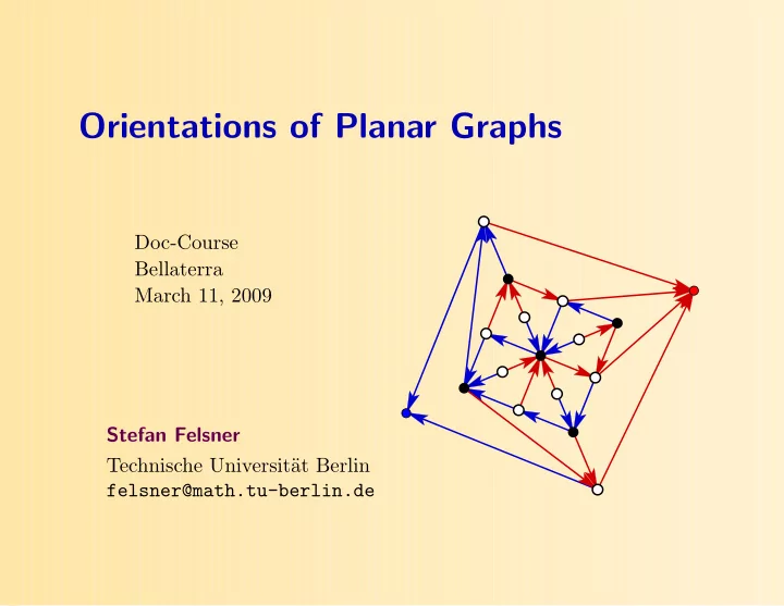
Doc-Course Bellaterra March 11, 2009 Stefan Felsner Technische Universit¨ at Berlin felsner@math.tu-berlin.de
Orientations of Planar Graphs Doc-Course Bellaterra March 11, 2009 - - PowerPoint PPT Presentation
Orientations of Planar Graphs Doc-Course Bellaterra March 11, 2009 Stefan Felsner Technische Universit at Berlin felsner@math.tu-berlin.de Topics -Orientations Sample Applications Counting I: Bounds Counting II: Exact Lattices
Doc-Course Bellaterra March 11, 2009 Stefan Felsner Technische Universit¨ at Berlin felsner@math.tu-berlin.de
α-Orientations Sample Applications Counting I: Bounds Counting II: Exact Lattices Counting III: Random Sampling
An α-orientation of G is an orientation with
Example. Two orientations for the same α.
i.e. α(v) = d(v)
2
G a planar graph. Spanning trees of G are in bijection with αT orientations of a rooted primal-dual completion G
an edge-vertex ve and αT(vr) = 0 and αT(v∗
r) = 0.
v∗
r
vr
G a planar triangulation, let
G a planar quadrangulation, let
α(v) = 2 for each other vertex. s t
α-Orientations
Counting I: Bounds Counting II: Exact Lattices Counting III: Random Sampling
G = (V, E) a plane triangulation, F = {a1,a2,a3} the outer triangle. A coloring and orientation of the interior edges of G with colors 1,2,3 is a Schnyder wood of G iff
Theorem. Schnyder woods and 3-orientations are equivalent. Proof.
→ ai is unique (again Euler).
common.
R1 R2 R3
v u
The count of faces in the green and red region yields two coordinates (vg, vr) for vertex v. = ⇒ straight line drawing on the 2n − 5 × 2n − 5 grid.
G = (V, E) a plane quadrangulation, F = {a0,x,a1,y} the outer face. A coloring and orientation of the interior edges of G with colors 0, 1 is a separating decomposition of G iff
color i.
Theorem. Separating decompositions and 2-orientations are equivalent. Proof.
The set Ti of edges colored i is a tree rooted at ai.
→ ai is unique.
common.
v u
The count of faces in the red region yields a number vr for vertex v = s, t. s t
with a unique source s and a unique sink t. s t
with a unique source s and a unique sink t. s t Plane bipolar orientations with s and t on the outer face are characterized by tf v f sf vertex face
s t s t A plane bipolar orientation and its angular map.
s t s t v-edges f-edges Angular edges oriented by vertices and faces.
A plane bipolar orientation and its dual orientation yield a rectangular layout (visibility representation). s t t′ s′ coordinates from longest paths
α-Orientations Sample Applications
Counting II: Exact Lattices Counting III: Random Sampling
Let G be a plane graph and α : V → IN. How many α-orientations can G have?
Let G be a plane graph and α : V → IN. How many α-orientations can G have? Choose a spanning tree T of G and orient the edges not in T randomly.
If at all the orientation on G − T is uniquely extendible. α ≡ 2 = ⇒ there are at most 2m−(n−1) α-orientations.
An orientation can be extended only if outdeg(v) ∈ {α(v), α(v) − 1} for all v. Let I be an independent set of size ≥ n
4 (4CT)
Choose a tree T such that I ⊂ leaves(T). Each v ∈ I can independently obstruct extendability. There are d(v)−1
α(v)
d(v)−1
α(v)−1
d(v)
α(v)
⌊d(v)/2⌋
for the orientations of edges at v.
Since Prob(d(v) = α(v)) ≤ 1 2d(v)−1
⌊d(v)/2⌋
4 we conclude:
2m−n 3 4 n/4 ≤ 22n 3 4 n/4 ≈ 3.73n
We show that there are many 3-orientation of the triangular lattice
Any subset of the green triangles can be flipped.
If 0 or 3 of the green neighbors are flipped a white triangle can be flipped. using Jensen’s ineq. = ⇒ # 3-orientations ≥ 2#f−green E(2f−white−flippable) ≥ 2n 2E(f−white−flippable) = 2n 2
2 8#f−white = 2 5 4n = 2.37n
α-Orientations Sample Applications Counting I: Bounds
Lattices Counting III: Random Sampling
alternating if it is a 1-book embedding with no double-arc. double arc
layout with the root as leftmost vertex. 1 2 3 4 5 6 7 8 9 1011 12 1314 15 1 2 3 4 5 6 7 8 9 10 15 14 13 12 11 Label black vertices at first visit, white vertices at last visit.
Proposition. The 2-book embedding induced by a separation decomposition splits into two alternating trees.
alternating trees on n vertices with reverse fingerprints and separating decompositions of quadrangulations with n + 2 vertices. S 0 0 1 1 1 T 1 1 0 0 1 T + rT rS S+
binary trees that preserves fingerprints. 0 1 1 1 0 1 0 1 1 1 1 0 0 1 0 1 1 1 0 1 0 1 1 1 1 0 0 1
binary trees with n leaves and reverse fingerprints and rectangular dissections∗ of the square based on n − 2 diagonal points.
∗This is again the rectangular layout associated to the bipolar orientation.
5 2 3 6 4 7 1 6 3 1 7 4 5 6 3 5 2 7 1 6 7 3 4 1 2 5 4 Max(π) Min(ρ(π)) 2
(Max(π), Min(π)) is a pair of binary trees with n leaves and reverse fingerprints.
3 − 14 − 2 and 2 − 41 − 3. Example: A non-Baxter permutation with a 2 − 41 − 3 pattern π = 6, 3, 8, 7, 2, 9, 1, 5, 4
→ (Max(π), Min(π)) is bijection between Baxter permutations of [n−1] and binary trees with n leaves and reverse fingerprints, i.e., rectangular dissections of the square based on n − 2 diagonal points.
Rule: If the south-corner of R(k) is a , i.e., a left child in tree T, then R(k − 1) is the next-left, otherwise, next-right.
Rule: If the south-corner of R(k) is a , i.e., a left child in tree T, then R(k − 1) is the next-left, otherwise, next-right. 6 7
Rule: If the south-corner of R(k) is a , i.e., a left child in tree T, then R(k − 1) is the next-left, otherwise, next-right. 6 7 5
Rule: If the south-corner of R(k) is a , i.e., a left child in tree T, then R(k − 1) is the next-left, otherwise, next-right. 6 4 7 5
Rule: If the south-corner of R(k) is a , i.e., a left child in tree T, then R(k − 1) is the next-left, otherwise, next-right. 6 4 3 7 5
Rule: If the south-corner of R(k) is a , i.e., a left child in tree T, then R(k − 1) is the next-left, otherwise, next-right. 4 3 6 2 1 6 1 3 2 4 2 4 3 6 1 5 7 7 5 5 7
α: Fingerprint extended by a leading 1 for left leaf. β: Inner nodes in in-order represented by 0 (left) and 1 (right) with the root being a 1. 0 1 1 1 0 1 0 1 1 1 1 0 0 1 1 1 1 1 1 1 1 0 0 1 1
α: Fingerprint including the left extreme leaf. β: Inner nodes in in-order represented by 0 (left) and 1 (right) with the root being a 1. Lemma.
n−1
αi =
n−1
βi and
k
αi ≥
k
βi 1 1 1 1 1 1 1 1
k
i=1 αi
= k
i=1 βi and
k+1
i=1 αi = k+1 i=1 βi determines the position of the root.
left leaves and j + 1 right leaves equals the number of nonintersecting lattice paths α′and β′ where: α′ : (0, 1) → (j, i + 1) β′ : (1, 0) → (j + 1, i) From the Lemma of Gessel Viennot we deduce that their number is det j+i
j
j−1
j+1
j
1 i + j + 1 i + j + 1 j i + j + 1 j + 1
number i of increases can be encoded by triples of disjoint lattice path. 0111 1 1111 0 0 0 0 0 0 0 1 11 11 1 1 1 11 11 11101 0
separating decompositions and 2-orientations on n + 2 vertices, rectangular dissections on n − 2 diagonal points .... is given by
n−2
2n!(n − 1)!(n − 2)! i!(i + 1)!(i + 2)!(n − i)!(n − i − 1)!(n − i − 2)! = 2 n(n − 1)2
n−2
n i n i + 1 n i + 2
with n + 3 vertices and bipolar orientations with n + 2 vertices and the special property: ⋆ The right side of every bounded face is of length two. a1 a3 a2 t s
Let T b and T r be the blue and red tree corresponding to a Schnyder wood. From (⋆′) we get some crucial properties
symbols (01)n ≤dom 1 + α.
Theorem [Bonichon]. The number of Schnyder woods on plane triangulations on n+3 vertices equals the pairs of non-crossing Dyck-path of length 2n which is Cn+2Cn − C2
n+1.
α-Orientations Sample Applications Counting I: Bounds Counting II: Exact
Counting III: Random Sampling
has the structure of a distributive lattice. Example.
along cycles. Theorem [Propp 1993]. The set of all orientations of a graph G with prescribed flow- differences for all cycles has the structure of a distributive lattice.
Theorem [Khuller, Naor and Klein 1993]. The set of all integral flows respecting capacity constraints (ℓ(e) ≤ f(e) ≤ u(e)) of a planar graph has the structure of a distributive lattice. 0 ≤ f(e) ≤ 1
∆-Bonds G = (V, E) a connected graph with a prescribed orientation. With x ∈ Z ZE and C cycle we define the circular flow difference ∆x(C) :=
x(e) −
x(e). With ∆ ∈ Z ZC and ℓ, u ∈ Z ZE let BG(∆, ℓ, u) be the set of x ∈ Z ZE such that ∆x = ∆ and ℓ ≤ x ≤ u. Theorem [Felsner, Knauer 2007]. BG(∆, ℓ, u) is a distributive lattice. The cover relation is vertex pushing.
∆-Bonds as Generalization BG(∆, ℓ, u) is the set of x ∈ IRE such that
Special cases:
(∆(C) = |C+| − c(C)).
(G∗ the dual of G).
A coloring of the edges of a digraph is a D-coloring iff
Theorem. A digraph D is connected, acyclic and admits a D-coloring ⇐ ⇒ D is the diagram of a distributive lattice.
α-Orientations Sample Applications Counting I: Bounds Counting II: Exact Lattices
Problem.
#P-complete?
#P-complete?
polynomial equivalent for self-reducible problems.
uniform sampling is the Markov Chain Monte Carlo method (MCMC).
particularly nice instance of MCMC. It allows exact uniform sampling via Coupling From The Past (CfP).
scheme for counting perfect matchings of bipartite graphs (Jerrum, Sinclair, and Vigoda 2001) can be used for approximate counting of α-orientations.
scheme for counting perfect matchings of bipartite graphs (Jerrum, Sinclair, and Vigoda 2001) can be used for approximate counting of α-orientations. But what about the lattice walk?
a polynomial convergence to the uniform distribution. Dyer, Frieze and Jerrum: Glauber dynamics is exponential for random bipartite graphs with min-degree ≥ 6.
a polynomial convergence to the uniform distribution. Dyer, Frieze and Jerrum: Glauber dynamics is exponential for random bipartite graphs with min-degree ≥ 6. In several situations where planarity plays a role rapid mixing could be proven:
Theorem [Fehrenbach 03]. Sampling Eulerian
grid using the LW Markov chain is polynomial. Theorem [Creed 05].
patches of the triangular grid using the LW Markov chain is polynomial.
Eulerian
patches
the triangular grid with holes using the LW Markov chain can be exponential.
Theorem [Fehrenbach 03]. Sampling Eulerian
grid using the LW Markov chain is polynomial. Theorem [Creed 05].
patches of the triangular grid using the LW Markov chain is polynomial.
Eulerian
patches
the triangular grid with holes using the LW Markov chain can be exponential. Problem. We do not know much about sampling α-orientations.