Optimization of Logical Queries Task: Consider the following - - PowerPoint PPT Presentation

Optimization of Logical Queries

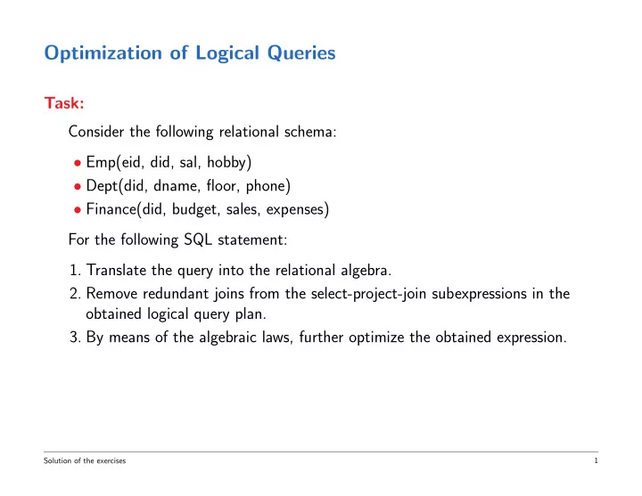
Task: Consider the following relational schema:

• Emp(eid, did, sal, hobby)
• Dept(did, dname, floor, phone)
• Finance(did, budget, sales, expenses)

For the following SQL statement:

• 1. Translate the query into the relational algebra.
• 2. Remove redundant joins from the select-project-join subexpressions in the
• btained logical query plan.
• 3. By means of the algebraic laws, further optimize the obtained expression.

Solution of the exercises 1

Optimization of Logical Queries

Task (continued)

SELECT D.floor FROM Dept D, Emp E WHERE (D.floor = 1 OR D.floor IN ( SELECT D2.floor FROM Dept D2, Finance F1 WHERE F1.budget > 150 AND D2.did = F1.did) ) AND E.did = D.did AND E.did IN (SELECT F2.did FROM Finance F2, Emp E2 WHERE F2.did = E.did AND E2.did = D.did AND E2.eid = E.eid AND F2.expenses = 300)

Solution of the exercises 2

Optimization of Logical Queries

Solution: translation into the relational algebra First, we normalize the query to a form with only EXISTS and NOT EXISTS subqueries:

SELECT D.floor FROM Dept D, Emp E WHERE (D.floor = 1 OR EXIST ( SELECT D2.floor FROM Dept D2, Finance F1 WHERE F1.budget > 150 AND D2.did = F1.did AND D2.floor = D.floor) ) AND E.did = D.did AND EXISTS (SELECT F2.did FROM Finance F2, Emp E2 WHERE F2.did = E.did AND E2.did = D.did AND E2.eid = E.eid AND F2.expenses = 300 AND E.did = F2.did)

Solution of the exercises 3

Optimization of Logical Queries

Conjunctive Normal Form

SELECT D.floor FROM Dept D, Emp E WHERE ( D.floor = 1 AND E.did = D.did AND EXISTS (SELECT F2.did FROM Finance F2, Emp E2 WHERE F2.did = E.did AND E2.did = D.did AND E2.eid = E.eid AND F2.expenses = 300 AND E.did = F2.did) ) OR ( EXIST ( SELECT D2.floor FROM Dept D2, Finance F1 WHERE F1.budget > 150 AND D2.did = F1.did AND D2.floor = D.floor) AND E.did = D.did AND EXISTS (SELECT F2.did FROM Finance F2, Emp E2 WHERE F2.did = E.did AND E2.did = D.did AND E2.eid = E.eid AND F2.expenses = 300 AND E.did = F2.did) )

Solution of the exercises 4

Optimization of Logical Queries

Normalize to UNION

Q1 = SELECT D.floor FROM Dept D, Emp E WHERE D.floor = 1 AND E.did = D.did AND EXISTS (SELECT F2.did FROM Finance F2, Emp E2 WHERE F2.did = E.did AND E2.did = D.did AND E2.eid = E.eid AND F2.expenses = 300 AND E.did = F2.did)

Solution of the exercises 5

Optimization of Logical Queries

Normalize to UNION

Q2 = SELECT D.floor FROM Dept D, Emp E WHERE EXIST ( SELECT D2.floor FROM Dept D2, Finance F1 WHERE F1.budget > 150 AND D2.did = F1.did AND D2.floor = D.floor) AND E.did = D.did AND EXISTS (SELECT F2.did FROM Finance F2, Emp E2 WHERE F2.did = E.did AND E2.did = D.did AND E2.eid = E.eid AND F2.expenses = 300 AND E.did = F2.did)

The new query is Q1 UNION Q2.

Solution of the exercises 6

Optimization of Logical Queries

Translation of the innermost subqueries

SELECT F2.did FROM Finance F2, Emp E2 WHERE F2.did = E.did AND E2.did = D.did AND E2.eid = E.eid AND F2.expenses = 300 AND E.did = F2.did

This subquery is translated as follows: e1 = πF2.did,E.∗,D.∗σF2.did=E.did∧E2.did=D.did∧E2.eid=E.eid σF2.expenses=300∧E.did=F2.did(ρD(Dept)×ρE(Emp)×ρF2(Finance)×ρE2(Emp))

Solution of the exercises 7

Optimization of Logical Queries

Translation of the innermost subqueries

SELECT D2.floor FROM Dept D2, Finance F1 WHERE F1.budget > 150 AND D2.did = F1.did AND D2.floor = D.floor

This subquery is translated as follows: e2 = πD2.floor,D.∗σF1.budget>150∧D2.did=F1.did σD2.floor=D.floor(ρD(Dept) × ρD2(Dept) × ρF1(Finance))

Solution of the exercises 8

Optimization of Logical Queries

Translation of the Middle Queries

Q1 = SELECT D.floor FROM Dept D, Emp E WHERE D.floor = 1 AND E.did = D.did AND EXISTS (SELECT F2.did FROM Finance F2, Emp E2 WHERE F2.did = E.did AND E2.did = D.did AND E2.eid = E.eid AND F2.expenses = 300 AND E.did = F2.did)

The translation of the from part gives e3 = (ρD(Dept) × ρE(Emp)) To de-correlate we compute: f = ˆ e3 ⋊ ⋉ πD.∗,E.∗(e1) Note that ˆ e3 is empty and hence f = πD.∗,E.∗(e1) To this expression we add the WHERE and SELECT clause: e4 = πD.floor(σD.floor=1∧E.did=D.did(πD.∗,E.∗(e1))

Solution of the exercises 9

Optimization of Logical Queries

Translation of the Middle Queries

Q2 = SELECT D.floor FROM Dept D, Emp E WHERE EXIST ( SELECT D2.floor FROM Dept D2, Finance F1 WHERE F1.budget > 150 AND D2.did = F1.did AND D2.floor = D.floor) AND E.did = D.did AND EXISTS (SELECT F2.did FROM Finance F2, Emp E2 WHERE F2.did = E.did AND E2.did = D.did AND E2.eid = E.eid AND F2.expenses = 300 AND E.did = F2.did)

The translation of the from part gives e5 = (ρD(Dept) × ρE(Emp)) To de-correlate we compute: f ′ = ˆ e5 ⋊ ⋉ (πD.∗,E.∗(e1) ⋊ ⋉ πD.∗(e2)) = (πD.∗,E.∗(e1) ⋊ ⋉ πD.∗(e2))

Solution of the exercises 10

To this expression we add the WHERE and SELECT clause: e6 = πD.floorσE.did=D.did(πD.∗,E.∗(e1) ⋊ ⋉ πD.∗(e2))

Solution of the exercises 11

Optimization of Logical Queries

Translation of the Whole Query

Q1 UNION Q2

Since the schemas of e4 and e6 are the same, the union is straightforward: e = e4 ∪ e6 Written in full: e = πD.floorσD.floor=1∧E.did=D.did πD.∗,E.∗σF2.did=E.did∧E2.did=D.did∧E2.eid=E.eid∧F2.expenses=300∧E.did=F2.did (ρD(Dept) × ρE(Emp) × ρF2(Finance) × ρE2(Emp)) ∪ πD.floorσE.did=D.did( [πD.∗,E.∗σF2.did=E.did∧E2.did=D.did∧E2.eid=E.eid∧F2.expenses=300∧E.did=F2.did (ρD(Dept) × ρE(Emp) × ρF2(Finance) × ρE2(Emp))] ⋊ ⋉ [πD.∗σF1.budget>150∧D2.did=F1.did∧D2.floor=D.floor (ρD(Dept) × ρD2(Dept) × ρF1(Finance))])

Solution of the exercises 12

Optimization of Logical Queries

Redundant Joins Removal The query comprises the following maximal select-project-join subexpressions:

• πD.floorσD.floor=1∧E.did=D.didπD.∗,E.∗σ...(ρD(Dept) × ρE(Emp) ×

ρF2(Finance) × ρE2(Emp))

• [πD.∗,E.∗σ...(ρD(Dept) × ρE(Emp) × ρF2(Finance) × ρE2(Emp))]
• (ρD(Dept) × ρD2(Dept) × ρF1(Finance))

Note that “F1.budget > 150” cannot be included in a select-project-join

• expression. Also note that the third expression does not contain redundant joins

(Why?).

Solution of the exercises 13

Optimization of Logical Queries

Redundant Joins Removal The first expression corresponds to: Q1(“1”) ←Dept(a1, a2, “1”, a4), Emp(b1, a1, b3, b4), Finance(a1, c2, c3, “300”), Emp(b1, a1, d3, d4) The first and third atoms cannot be removed (Why?) We check whether we can remove the second atom: Q2(“1”) ← Dept(a1, a2, “1”, a4), Finance(a1, c2, c3, “300”), Emp(b1, a1, d3, d4) The corresponding canonical database: D2(“1”) = {Dept( ˙ a1, ˙ a2, “1”, ˙ a4), Finance( ˙ a1, ˙ c2, ˙ c3, “300”), Emp( ˙ b1, ˙ a1, ˙ d3, ˙ d4)} Clearly (“1”) ∈ Q1(D2) because of the matching a1 → ˙ a1 a2 → ˙ a2 a4 → ˙ a4 b1 → ˙ b1 b3 → ˙ d3 b4 → ˙ d4 c2 → ˙ c2 c3 → ˙ c3 d3 → ˙ d3 d4 → ˙ d4 hence Q2 ⊆ Q1. The other direction always holds. Hence Q1 ≡ Q2

Solution of the exercises 14

Optimization of Logical Queries

Redundant Joins Removal No other atom can be removed (Why?). The optimal query is hence Q2(“1”) ← Dept(a1, a2, “1”, a4), Finance(a1, c2, c3, “300”), Emp(b1, a1, d3, d4) Translating this query back to the relational algebra, we obtain: πD.floor([σD.floor=1∧E2.did=D.did∧F2.did=E2.did∧E2.did=D.did∧F2.expenses=300 (ρD(Dept) × ρF2(Finance) × ρE2(Emp))])

Solution of the exercises 15

Optimization of Logical Queries

Redundant Joins Removal The second expression is: [πD.∗,E.∗σF2.did=E.did∧E2.did=D.did∧E2.eid=E.eid∧F2.expenses=300∧E.did=F2.did (ρD(Dept) × ρE(Emp) × ρF2(Finance) × ρE2(Emp))] Translated: Q3(a1, a2, a3, a4, b1, b2, b3, b4) ←Dept(a1, a2, a3, a4), Emp(b1, b2, b3, b4), Finance(a1, c2, c3, “300”), Emp(b1, a1, d3, d4) We cannot remove the second atom, this time (why?)

Solution of the exercises 16

Optimization of Logical Queries

Redundant Joins Removal Let us try to remove the fourth atom, let Q4(a1, a2, a3, a4, b1, b2, b3, b4) ←Dept(a1, a2, a3, a4), Emp(b1, b2, b3, b4), Finance(a1, c2, c3, “300”) By evaluating Q3 on the canonical database of Q4 we see that Q4 ⊆ Q3. Hence Q3 ≡ Q4 and the fourth atom can hence not be removed. This original SPJ expression was hence optimal.

Solution of the exercises 17

Optimization of Logical Queries

Redundant Joins Removal The third expression is: (ρD(Dept) × ρD2(Dept) × ρF1(Finance)) Translated: Q5(a1, . . . , a4, b1, . . . , b4, c1, . . . , c4) ←Dept(a1, a2, a3, a4), Dept(b1, b2, b3, b4), Finance(c1, c2, c3, c4) No atoms can be removed (why?)

Solution of the exercises 18

Optimization of Logical Queries

Redundant Joins Removal The optimized expression is therefore: e = πD.floor([σD.floor=1∧E2.did=D.did∧F2.did=E2.did∧E2.did=D.did∧F2.expenses=300 (ρD(Dept) × ρF2(Finance) × ρE2(Emp))]) ∪ πD.floorσE.did=D.did( [πD.∗,E.∗σF2.did=E.did∧E2.did=D.did∧E2.eid=E.eid∧F2.expenses=300∧E.did=F2.did (ρD(Dept) × ρE(Emp) × ρF2(Finance) × ρE2(Emp))] ⋊ ⋉ [πD.∗σF1.budget>150∧D2.did=F1.did∧D2.floor=D.floor (ρD(Dept) × ρD2(Dept) × ρF1(Finance))])

Solution of the exercises 19

Cost-based plan selection

Task (refer to the handouts for the full exercise) Construct a sufficiently optimal physical query plan for: πE.eid,D.did,P.pidσE.sal=50000(E) ⋊ ⋉ σD.budget≥20000(D) ⋊ ⋉ P Assume that employee salaries are uniformly distributed over the range [10009, 110008] and that project budgets are uniformly distributed over [10000, 30000]. There are clustered indexes available on E.sal, D.did and P.pid.

Solution of the exercises 20

Cost-based plan selection

Solution π ⋊ ⋉ σ E σ D P

Solution of the exercises 21

Cost-based plan selection

Solution π ⋊ ⋉ σ E σ D P

Solution of the exercises 22

Cost-based plan selection

Solution Subexpression: σE.sal=50000(E) First possibility: we use the clustered index on E.sal to get the records such that E.sal = 50000. The number of tuples that satisfy the salary requirement is estimated to:

• 1

110008 − 10009 + 1 selectivity × 20000 employees

• = 1 tuples

Hence, the result can be stored in 1 block, which is also the cost of the index scan:

• 20 bytes

4000 bytes/block

• = 1 block

Solution of the exercises 23

Cost-based plan selection

Solution Subexpression: σE.sal=50000(E) Second possibility: we use a table scan, which costs 20000 tuples

• 4000 bytes/block

20 bytes/tuple

= 100 block I/Os Clearly, we prefer the index scan. Pipelining: since selections can be pipelined, we (greedily) decide to pipeline this seclection

Solution of the exercises 24

Cost-based plan selection

Solution π ⋊ ⋉ σ E σ D P T = 1 B = 1

Solution of the exercises 25

Cost-based plan selection

Solution π ⋊ ⋉ σ E σ D P

Solution of the exercises 26

Cost-based plan selection

Solution Subexpression: σD.budget≥20000(D) The number of tuples returned is estimated to 2501: 30000 − 20000 + 1 30000 − 10000 + 1 selectivity × 5000 departments

• = 2501 tuples

This corresponds to 26 Blocks: 2501

• 4000 bytes/block

40 bytes/tuple

= 26 blocks Since no index is available, a table scan is our only possibility: 5000

• 4000 bytes/block

40 bytes/tuple

= 50 blocks Pipelining: since selections can be pipelined, we (greedily) decide to pipeline this seclection

Solution of the exercises 27

Cost-based plan selection

Solution π ⋊ ⋉ σ E σ D P T = 2501 B = 26

Solution of the exercises 28

Cost-based plan selection

Solution π ⋊ ⋉ σ E σ D P

Solution of the exercises 29

Cost-based plan selection

Solution Subexpression: P A table scan on P requires 500 block I/O’s. This is also the estimated number

• f blocks returned:

1000 tuples

• 4000 bytes/block

2000 bytes/tuple

= 500 blocks

Solution of the exercises 30

Cost-based plan selection

Solution π ⋊ ⋉ σ E σ D P T = 1000 B = 500

Solution of the exercises 31

Cost-based plan selection

Solution π ⋊ ⋉ σ E σ D P π ⋊ ⋉ ⋊ ⋉ σ E σ D P π ⋊ ⋉ σ E ⋊ ⋉ σ D P π ⋊ ⋉ σ D ⋊ ⋉ σ E P

Solution of the exercises 32

Cost-based plan selection

Solution Now, we must determine an ordering for the joins. We consider all pairs of joins and keep the one with the smallest cost. σe.sal=50000(E)

• e1

and σd.budget≥20000(D)

• e2

The selection on each side requires one buffer to execute, leaving only 10 buffers for the join. The output of e1 contains only 1 tuples, and can therefore be computed in 1

• block. Since 1 = B(e1) ≤ M = 10, we can apply the one-pass join algorithm.

Its cost is B(e1) + B(e2) = 1 + 26 = 27 I/O’s An index-join cannot be used on e2 since it is not a base relation. All other join methods always cost more than one-pass join. Hence the one-pass join is preferred.

Solution of the exercises 33

Cost-based plan selection

Solution π ⋊ ⋉ σ E σ D P π ⋊ ⋉ ⋊ ⋉ σ E σ D P π ⋊ ⋉ σ E ⋊ ⋉ σ D P π ⋊ ⋉ σ D ⋊ ⋉ σ E P

Solution of the exercises 34

Cost-based plan selection

Solution The second join pair is: σD.budget≥20000(D)

• e2

and P We have 11 buffers at our disposal, given that we need 1 buffer to perform the selection in e2. It is not possible to use a one-pass join, since 26 = B(e2) ≥ M = 11 and 500 = B(P) ≥ M = 11. A block-based nested-loop join costs: B(e2) + B(e2) M − 1

• × B(P) = 26 +

26 10

• × 500 = 1526 I/Os

Solution of the exercises 35

Cost-based plan selection

Solution The second join pair is: σD.budget≥20000(D)

• e2

and P We have enough memory to perform an optimized sort-merge join: 8 =

• B(e2)

M ⌈logM B(e2)⌉−1

• +
• B(P)

M ⌈logM B(P)⌉−1

• ≤ M = 11 available buffers

This optimized sort-merge join has a cost of: 2B(e2) ⌈logM B(e2)⌉ + 2B(P) ⌈logM B(P)⌉ − B(e2) − B(P) = 2 × 26 × 2 + 2 × 500 × 3 − 26 − 500 = 2578 I/O’s

Solution of the exercises 36

Cost-based plan selection

Solution Assuming that the clustered index on P.pid is a BTree, it ensues that P is already sorted on this join attribute. Given that we then only need to sort e2, the cost of a non-optimized sort-merge join is: 2B(e2) ⌈logM B(e2)⌉ + B(e2) + B(P) Futhermore, we can optimize the last merge: 4 necessary buffers = B(e2) M

• + 1 ≤ M = 11 available buffers

The cost thereof is: 2B(e2)(⌈logM B(e2)⌉ − 1) + B(e2) + B(P) = 2 × 26 × 1 + 26 + 500 = 578 I/Os

Solution of the exercises 37

Cost-based plan selection

Solution The cost of an hash-join is: 2B(e2) ⌈logM−1 B(e2) − 1⌉ + 2B(P) ⌈logM−1 B(e2) − 1⌉ + B(e2) + B(P) = 2 × 26 × 1 + 2 × 500 × 1 + 26 + 500 = 1578 I/O’s It is also possible to use an index-join, using the clustered index on P.pid. This method has a cost of: B(e2) + T(e2) ×

• B(P)

V (P, pid)

• = 26 + 2501 × 1 = 2527 I/O’s

Hence, we assume that the index on P.pid is a BTree, and sorting P is not

• necessary. In that case the optimized sort-merge join that only sorts e2 is

preferred.

Solution of the exercises 38

Cost-based plan selection

Solution π ⋊ ⋉ σ E σ D P π ⋊ ⋉ ⋊ ⋉ σ E σ D P π ⋊ ⋉ σ E ⋊ ⋉ σ D P π ⋊ ⋉ σ D ⋊ ⋉ σ E P

Solution of the exercises 39

Cost-based plan selection

Solution The third join pair is: σE.sal=50000(E)

• e1

and P Note that this join is a full cartesian product. A one-pass join is available at the following cost: B(e1) + B(P) = 1 + 500 = 501 I/O’s No index can help up for this join, and the one-pass join algorithm gives the best cost.

Solution of the exercises 40

Cost-based plan selection

Solution π ⋊ ⋉ σ E σ D P π ⋊ ⋉ ⋊ ⋉ σ E σ D P π ⋊ ⋉ σ E ⋊ ⋉ σ D P π ⋊ ⋉ σ D ⋊ ⋉ σ E P Cost = 27 Single pass join Cost = 578 Optimized sort-merge join Cost = 501 Single pass join

Solution of the exercises 41

Cost-based plan selection

Solution The join-pair with the least cost is therefore: σe.sal=50000(E)

• e1

and σD.budget≥20000(D)

• e2

Where an one-pass join on E.did is used. This one-pass join computes in-memory the result of e1, and iterates block-by block over the results of e2. Therefore, only 2 buffers are necessary (why?). We greedily decide that the output of this join is pipelined to the next operator. The estimated number of tuples in the output of this join is: T(e1) × T(e2) max(V (e1, did), V (e2, did)) = 1 × 2501 20 = 126 These records are 60 bytes long and can be stored in 2 blocks

Solution of the exercises 42

Cost-based plan selection

Solution π ⋊ ⋉ ⋊ ⋉ σ E σ D P T = 126 B = 2

Solution of the exercises 43

Cost-based plan selection

Solution π ⋊ ⋉ ⋊ ⋉ σ E σ D P

Solution of the exercises 44

Cost-based plan selection

Solution We still need to find the best way to join the whole expression σe.sal=50000(E) ⋊ ⋉ σD.budget≥20000(D)

• e3

and P We expect to have 12 − 2 = 10 main memory buffers available. The output of e3 fits in 2 blocks. Given that 2 = B(e3) ≤ M = 10, a one-pass join is possible. The cost thereof is: B(e3) + B(P) = 2 + 500 = 502 This join can also be performed by means of an index-join, using the clustered index on P.pid. B(e3) + T(e3) ×

• B(P)

V (P, pid)

• = 2 + 125 × 1 = 127 I/O’s

Hence, the index-join is preferred. We greedily decide to pipeline this join.

Solution of the exercises 45

Cost-based plan selection

Solution π ⋊ ⋉ ⋊ ⋉ σ E σ D P

Solution of the exercises 46

Cost-based plan selection

Solution The projection πE.eid,D.did,P.pid can be performed on the fly at the same time as the last join. Notice that we did not need to materialize any of the intermediate results.

Solution of the exercises 47

Cost-based plan selection

Solution π ⋊ ⋉ ⋊ ⋉ σ E σ D P Index join Cost = 127, T = 125 Single pass Cost = 27, T = 126 Table scan Cost = 50, T = 2501 Index scan Cost = 1, T = 1

Solution of the exercises 48