optimal filter and cost benefit analysis
play

Optimal filter and Cost-Benefit Analysis Tyler Moore CSE 7338 - PDF document

Notes Optimal filter and Cost-Benefit Analysis Tyler Moore CSE 7338 Computer Science & Engineering Department, SMU, Dallas, TX Lecture 3 Notes Outline Information security risk management 1 Optimal filter configuration 2 Cost-benefit


  1. Notes Optimal filter and Cost-Benefit Analysis Tyler Moore CSE 7338 Computer Science & Engineering Department, SMU, Dallas, TX Lecture 3 Notes Outline Information security risk management 1 Optimal filter configuration 2 Cost-benefit analysis 3 2 / 53 Information security risk management Notes Information security risk management Just as it can be useful to translate infosec risks and defenses into the language of investment (ROSI, NPV, etc.), one must also be aware of terminology from risk management As IT becomes essential to many businesses, border between information security investment and general risk management has blurred 4 / 53 Information security risk management Notes 
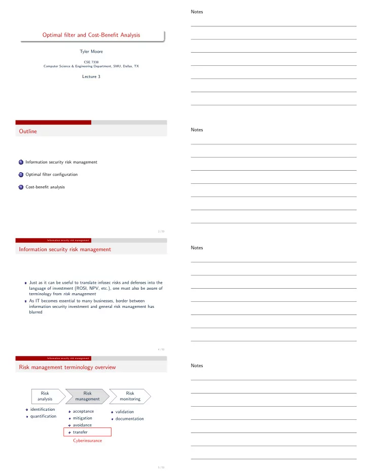
Risk management terminology overview Risk Risk Risk analysis management monitoring identification acceptance validation quantification mitigation documentation avoidance transfer Cyberinsurance 5 / 53

  2. Information security risk management Risk acceptance Notes Risk acceptance After risks are identified and quantified, they must be “managed” The simplest option is to do nothing Such “risk acceptance” is prudent when: Worst-case loss is small enough to be paid from proceeds or reserves 1 Probability of occurrence is smaller than other business risks that 2 threaten the organization’s survival This is why the security policies for start-ups are often weaker than for entrenched firms 6 / 53 Information security risk management Risk mitigation Notes Risk mitigation If risk is too big and probable to be accepted, risk mitigation aims to reduce the probability and severity of a loss This is where security investment comes in Recall that the optimal level of investment normally leaves residual risk that must be dealt with using acceptance, avoidance, or transfer 7 / 53 Information security risk management Risk avoidance Notes Risk avoidance Aims to reduce the probability and severity of loss, as in risk mitigation However, rather than use technology, here one forgoes risky activities This introduces opportunity costs of lost business opportunities Example: online merchant refusing overseas orders due to high fraud risk Example: company disconnects database with customers’ personal information online Question: what are the opportunity costs in these cases? 8 / 53 Information security risk management Risk avoidance Notes Risk transfer The final option is to buy an insurance contract to recover any future losses incurred This is only available in limited circumstances Why has the cyber-insurance market remained small? Difficulty in quantifying losses Even when possible, many firms would rather keep quiet than share with an insurance company Externalities mean that the costs of insecurity are often borne by others Correlated risk is prevalent 9 / 53

  3. Information security risk management Risk avoidance Notes Risk management example: credit card issuers Credit card issuers regularly manage fraud 1 Risk acceptance: fraud is paid from the payment fees charged to merchants 2 Risk mitigation: install anti-fraud technology (raises costs of security) 3 Risk avoidance: downgrade high-risk cardholders to debit or require online verification (leads to lost business) 4 Risk transfer: structure consumer credit risk and sell it on the market 10 / 53 Optimal filter configuration Notes Domain-specific models Up to now we have modeled security investment at a very high level Map costs to benefits, assume diminishing marginal returns to investment, etc. Useful for when justifying security budgets compared to non-security expenditures Not useful for deciding how best to allocate a given security budget Today, we discuss a model for a tactical security investment decision: configuring a filter to balance false positives and negatives 12 / 53 Optimal filter configuration ROC curves Notes Binary classification is a recurring problem in CS Common task: distill many observations to a binary signal { 0 , 1 } : communications theory S = { undervalued , overvalued } : stock trading S = { reject , accept } : research hypothesis S = { benign , malicious } : security filter Such simplification inevitably leads to errors compared to reality (aka ground truth ) 13 / 53 Optimal filter configuration ROC curves Notes Filter defense mechanism Reality Signal no attack attack benign 1 − α β malicious α 1 − β α : false positive rate, β : false negative rate 14 / 53

  4. Optimal filter configuration ROC curves Notes Receiver operating characteristic 1 Detection rate 1 − β 45 ◦ 0 1 False positive rate α 15 / 53 Optimal filter configuration ROC curves Notes Receiver operating characteristic 1 Detection rate 1 − β α = β 45 ◦ 0 1 EER dashed EER solid False positive rate α 15 / 53 Optimal filter configuration An economic model of optimal filter configuration Notes Model for optimal filter configuration Binary classifiers are imperfect Finding the optimal trade-off, say for an IDS or spam filter, is hard Can be framed as an economic trade-off between opportunity cost of false positives and losses incurred by false negatives 16 / 53 Optimal filter configuration An economic model of optimal filter configuration Notes Model for optimal filter configuration We can see from ROCs that β can be expressed as a function of α . β : [0 , 1] → [0 , 1] defines the false negative rate as a function of the false positive rate α β (0) = 1 , β (1) = 0 We assume β ′ ( x ) < 0 and β ′′ ( x ) ≥ 0 17 / 53

  5. Optimal filter configuration An economic model of optimal filter configuration Notes Model for optimal filter configuration Suppose we rely on a filter to scan incoming email attachments for malware a : cost of false positive (blocking a benign email) b : cost of false negative (delivering malicious email) p : probability of email containing malware Cost C ( α ) = p · β ( α ) · b + (1 − p ) · α · a Suppose p = 0 . 1 , a = $250 , b = $500 , α = 0 . 1 , β = . 2 C ( α ) = 0 . 1 · 0 . 2 · 500 + 0 . 9 · 0 . 1 · 250 = $32 . 50 18 / 53 Optimal filter configuration An economic model of optimal filter configuration Notes Optimal filter configuration: exercise 1 Suppose we rely on a filter to scan incoming email attachments for malware. Suppose the cost of dealing with a false negative event is $400, and the cost of dealing with a false positive is $200. 20% of incoming email has malware. You can choose between two configurations Config. A: 10% false positive rate and 30% false negative rate Config. B: 25% false positive rate and 15% false negative rate Your task: compute the expected costs for both configurations, and state which configuration you prefer. 19 / 53 Optimal filter configuration An economic model of optimal filter configuration Notes Model for optimal filter configuration α ∗ = arg min α p · β ( α ) · b + (1 − p ) · α · a which has first-order condition (FOC) p · β ( α ∗ ) · b + (1 − p ) · α ∗ · a 0 = δ α � � after rearranging, we obtain: β ′ ( α ∗ ) = − 1 − p · a p b 20 / 53 Optimal filter configuration An economic model of optimal filter configuration Notes Optimal filter configuration (continuous ROC curves) 1 (1 − p ) a p · b Detection rate 1 − β α ∗ B Indifference curves α ∗ A 0 False positive rate α 1 21 / 53

  6. Optimal filter configuration An economic model of optimal filter configuration Notes Optimal filter configuration (continuous ROC curves) 1 A B Detection rate 1 − β EER A = EER B α = β AUC A = AUC B 45 ◦ 0 False positive rate α 1 21 / 53 Optimal filter configuration An economic model of optimal filter configuration Notes Optimal filter configuration (continuous ROC curves) 1 A B (1 − p ) a p · b Detection rate 1 − β α ∗ B α ∗ A 45 ◦ 0 False positive rate α 1 21 / 53 Optimal filter configuration An economic model of optimal filter configuration Notes Optimal filter configuration (discrete ROC curves) 1 E F (1 − p ) a p · b Detection rate 1 − β α ∗ D 45 ◦ C 0 False positive rate α 1 22 / 53 Optimal filter configuration An economic model of optimal filter configuration Notes Optimal filter configuration example (discrete ROC curves) slope 1/3 1 E F 0.1 0.3 0.9 Detection rate 1 − β (1 − p ) a p · b 1 0.5 e p o l s α ∗ D 0.5 0.4 2 α ∗ = 0 . 2 if 1 ≤ (1 − p ) a ≤ 2 e 0.4 p p · b o l s C 0.2 0.2 0.7 0 1 False positive rate α 23 / 53

Download Presentation
Download Policy: The content available on the website is offered to you 'AS IS' for your personal information and use only. It cannot be commercialized, licensed, or distributed on other websites without prior consent from the author. To download a presentation, simply click this link. If you encounter any difficulties during the download process, it's possible that the publisher has removed the file from their server.

Recommend


More recommend