
SLIDE 1
On a prey-predator model
Igor Kortchemski
CNRS & CMAP, École polytechnique
Bonn probability seminar – July 2015
On a prey-predator model Igor Kortchemski CNRS & CMAP, cole - - PowerPoint PPT Presentation
On a prey-predator model Igor Kortchemski CNRS & CMAP, cole polytechnique Bonn probability seminar July 2015 Test your intuition! Complete graphs Infinite trees What is this about? On a graph, we are interested in the following
Igor Kortchemski
CNRS & CMAP, École polytechnique
Bonn probability seminar – July 2015
Test your intuition! Complete graphs Infinite trees
On a graph, we are interested in the following prey-predator model (introduced by Bordenave ’12) :
Igor Kortchemski Preys & Predators 1 / 5
Test your intuition! Complete graphs Infinite trees
On a graph, we are interested in the following prey-predator model (introduced by Bordenave ’12) :
Igor Kortchemski Preys & Predators 1 / 5
Test your intuition! Complete graphs Infinite trees
On a graph, we are interested in the following prey-predator model (introduced by Bordenave ’12) :
Igor Kortchemski Preys & Predators 1 / 5
Test your intuition! Complete graphs Infinite trees
On a graph, we are interested in the following prey-predator model (introduced by Bordenave ’12) :
Igor Kortchemski Preys & Predators 1 / 5
Test your intuition! Complete graphs Infinite trees
On a graph, we are interested in the following prey-predator model (introduced by Bordenave ’12) :
Motivations : Model of two competing species, or model of first-passage percolation with destruction.
Igor Kortchemski Preys & Predators 1 / 5
Test your intuition! Complete graphs Infinite trees
On a graph, we are interested in the following prey-predator model (introduced by Bordenave ’12) :
Motivations : Model of two competing species, or model of first-passage percolation with destruction. Other possible analogies: vacant vertex ⇐ ⇒ prey ⇐ ⇒ predator ⇐ ⇒
Igor Kortchemski Preys & Predators 1 / 5
Test your intuition! Complete graphs Infinite trees
On a graph, we are interested in the following prey-predator model (introduced by Bordenave ’12) :
Motivations : Model of two competing species, or model of first-passage percolation with destruction. Other possible analogies: vacant vertex ⇐ ⇒ vacant vertex prey ⇐ ⇒ healthy cell predator ⇐ ⇒ cell infected by a virus
Igor Kortchemski Preys & Predators 1 / 5
Test your intuition! Complete graphs Infinite trees
On a graph, we are interested in the following prey-predator model (introduced by Bordenave ’12) :
Motivations : Model of two competing species, or model of first-passage percolation with destruction. Other possible analogies: vacant vertex ⇐ ⇒ normal individual prey ⇐ ⇒ individual trying to spread a rumor (spreader) predator ⇐ ⇒ individual trying to scotch the rumor (stifler)
Igor Kortchemski Preys & Predators 1 / 5
Test your intuition! Complete graphs Infinite trees
On a graph, we are interested in the following prey-predator model (introduced by Bordenave ’12) :
Motivations : Model of two competing species, or model of first-passage percolation with destruction. Other possible analogies: vacant vertex ⇐ ⇒ Susceptible (S) individual prey ⇐ ⇒ Infected (I) individual predator ⇐ ⇒ Recovered (R) individual
Igor Kortchemski Preys & Predators 1 / 5
Test your intuition! Complete graphs Infinite trees
Here, {I, S}
λ
→ {I, I}, {R, I}
1
→ {R, R}. Other type of models studied in the literature:
Igor Kortchemski Preys & Predators 2 / 5
Test your intuition! Complete graphs Infinite trees
Here, {I, S}
λ
→ {I, I}, {R, I}
1
→ {R, R}. Other type of models studied in the literature: – SIR model (Kermack—McKendrick ’27), where {I, S}
λ
→ {I, I}, I
1
→ R
Igor Kortchemski Preys & Predators 2 / 5
Test your intuition! Complete graphs Infinite trees
Here, {I, S}
λ
→ {I, I}, {R, I}
1
→ {R, R}. Other type of models studied in the literature: – SIR model (Kermack—McKendrick ’27), where {I, S}
λ
→ {I, I}, I
1
→ R – Daley–Kendall (’65) rumour propagation model, where {I, S}
1
→ {I, I}, {R, I}
1
→ {R, R}, {I, I}
1
→ {R, R}.
Igor Kortchemski Preys & Predators 2 / 5
Test your intuition! Complete graphs Infinite trees
Here, {I, S}
λ
→ {I, I}, {R, I}
1
→ {R, R}. Other type of models studied in the literature: – SIR model (Kermack—McKendrick ’27), where {I, S}
λ
→ {I, I}, I
1
→ R – Daley–Kendall (’65) rumour propagation model, where {I, S}
1
→ {I, I}, {R, I}
1
→ {R, R}, {I, I}
1
→ {R, R}. – Maki–Thompson (’73) directed rumour propagation model, where (I, S)
1
→ (I, I), (R, I)
1
→ (R, R), (I, I)
1
→ (I, R).
Igor Kortchemski Preys & Predators 2 / 5
Test your intuition! Complete graphs Infinite trees
Here, {I, S}
λ
→ {I, I}, {R, I}
1
→ {R, R}. Other type of models studied in the literature: – SIR model (Kermack—McKendrick ’27), where {I, S}
λ
→ {I, I}, I
1
→ R – Daley–Kendall (’65) rumour propagation model, where {I, S}
1
→ {I, I}, {R, I}
1
→ {R, R}, {I, I}
1
→ {R, R}. – Maki–Thompson (’73) directed rumour propagation model, where (I, S)
1
→ (I, I), (R, I)
1
→ (R, R), (I, I)
1
→ (I, R). – Williams Bjerknes (’71) tumor growth model (or biased voter model), where (I, S)
λ
→ (I, I), (S, I)
1
→ (S, S).
Igor Kortchemski Preys & Predators 2 / 5
Test your intuition! Complete graphs Infinite trees
Here, {I, S}
λ
→ {I, I}, {R, I}
1
→ {R, R}. Other type of models studied in the literature: – SIR model (Kermack—McKendrick ’27), where {I, S}
λ
→ {I, I}, I
1
→ R – Daley–Kendall (’65) rumour propagation model, where {I, S}
1
→ {I, I}, {R, I}
1
→ {R, R}, {I, I}
1
→ {R, R}. – Maki–Thompson (’73) directed rumour propagation model, where (I, S)
1
→ (I, I), (R, I)
1
→ (R, R), (I, I)
1
→ (I, R). – Williams Bjerknes (’71) tumor growth model (or biased voter model), where (I, S)
λ
→ (I, I), (S, I)
1
→ (S, S). – Kordzakhia (’05), where {I, S}
λ
→ {I, I}, {R, I}
1
→ {R, R}, {R, S}
1
→ {R, R}.
Igor Kortchemski Preys & Predators 2 / 5
Test your intuition! Complete graphs Infinite trees
Igor Kortchemski Preys & Predators 3 / 5
Test your intuition! Complete graphs Infinite trees
Igor Kortchemski Preys & Predators 3 / 5
Test your intuition! Complete graphs Infinite trees
Igor Kortchemski Preys & Predators 3 / 5
Test your intuition! Complete graphs Infinite trees
Igor Kortchemski Preys & Predators 4 / 5
Test your intuition! Complete graphs Infinite trees
You have a box with n red balls and n blue balls.
Igor Kortchemski Preys & Predators 5 / 465
Test your intuition! Complete graphs Infinite trees
You have a box with n red balls and n blue balls. You take out each time a ball at random.
Igor Kortchemski Preys & Predators 5 / 465
Test your intuition! Complete graphs Infinite trees
You have a box with n red balls and n blue balls. You take out each time a ball at random. If the ball was red, you put it back in the box and take out a blue ball.
Igor Kortchemski Preys & Predators 5 / 465
Test your intuition! Complete graphs Infinite trees
You have a box with n red balls and n blue balls. You take out each time a ball at random. If the ball was red, you put it back in the box and take out a blue
Igor Kortchemski Preys & Predators 5 / 465
Test your intuition! Complete graphs Infinite trees
You have a box with n red balls and n blue balls. You take out each time a ball at random. If the ball was red, you put it back in the box and take out a blue
You keep doing it until left only with balls of the same color. How many balls will be left (as a function of n)?
Igor Kortchemski Preys & Predators 5 / 465
Test your intuition! Complete graphs Infinite trees
You have a box with n red balls and n blue balls. You take out each time a ball at random. If the ball was red, you put it back in the box and take out a blue
You keep doing it until left only with balls of the same color. How many balls will be left (as a function of n)? 1) Roughly ✏n for some ✏ > 0. 2) Roughly √n. 3) Roughly log n. 4) Roughly a constant. 5) Some other behavior.
Igor Kortchemski Preys & Predators 5 / 465
Test your intuition! Complete graphs Infinite trees
You have a box with n red balls and n blue balls. You take out each time a ball at random. If the ball was red, you put it back in the box and take out a blue
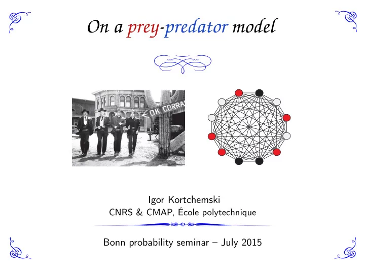
You keep doing it until left only with balls of the same color. How many balls will be left (as a function of n)? 1) Roughly ✏n for some ✏ > 0. 2) Roughly √n. 3) Roughly log n. 4) Roughly a constant. 5) Some other behavior. Other formulation (O.K. Corral problem, Williams & McIlroy, 1998) . There are two groups of n gunmen that shoot at each other. Once a gunman is hit he stops shooting, and leaves the place happily and peacefully. How many gunmen will be left after all gunmen in one team have left?
Igor Kortchemski Preys & Predators 5 / 465
Test your intuition! Complete graphs Infinite trees
Figure: Excerpt of the film “Gunfight at the O.K. Corral” (1957)
Igor Kortchemski Preys & Predators 6 / 465
Test your intuition! Complete graphs Infinite trees
You have a box with n red balls and n blue balls. You take out each time a ball at random. If the ball was red, you put it back in the box and take out a blue
You keep as before until left only with balls of the same color. How many balls will be left (as a function of n)? 1) Roughly ✏n for some ✏ > 0. 2) Roughly √n. 3) Roughly log n. 4) Roughly a constant. 5) Some other behavior. Other formulation (O.K. Corral problem, Williams & McIlroy, 1998) . There are two groups of n gunmen that shoot at each other. Once a gunman is hit he stops shooting, and leaves the place happily and peacefully. How many gunmen will be left after all gunmen in one team have left?
Igor Kortchemski Preys & Predators 7 / 465
Test your intuition! Complete graphs Infinite trees
If urn A has m balls and urn B has n balls, the probability that a ball is removed from A is
n m+n.
Igor Kortchemski Preys & Predators 8 / 465
Test your intuition! Complete graphs Infinite trees
If urn A has m balls and urn B has n balls, the probability that a ball is removed from A is
n m+n. But
n m + n = 1/m 1/m + 1/n = P (Exp(1/m) < Exp(1/n)) .
Igor Kortchemski Preys & Predators 8 / 465
Test your intuition! Complete graphs Infinite trees
Let (Xi, Yi)i>1 be independent random variables such that Xi are Yi exponential random variables with mean i.
Igor Kortchemski Preys & Predators 9 / 465
Test your intuition! Complete graphs Infinite trees
Let (Xi, Yi)i>1 be independent random variables such that Xi are Yi exponential random variables with mean i. Consider a piece of wood represented by the interval [−n, n] and made of 2n pieces such that length([i − 1, i]) = Xi, length([−i, −i + 1]) = Yi (1 6 i 6 n).
Igor Kortchemski Preys & Predators 9 / 465
Test your intuition! Complete graphs Infinite trees
Let (Xi, Yi)i>1 be independent random variables such that Xi are Yi exponential random variables with mean i. Consider a piece of wood represented by the interval [−n, n] and made of 2n pieces such that length([i − 1, i]) = Xi, length([−i, −i + 1]) = Yi (1 6 i 6 n). Light both ends, and stop the fire when the origin is reached.
Igor Kortchemski Preys & Predators 9 / 465
Test your intuition! Complete graphs Infinite trees
Let (Xi, Yi)i>1 be independent random variables such that Xi are Yi exponential random variables with mean i. Consider a piece of wood represented by the interval [−n, n] and made of 2n pieces such that length([i − 1, i]) = Xi, length([−i, −i + 1]) = Yi (1 6 i 6 n). Light both ends, and stop the fire when the origin is reached. Let R(n) be the number of remaining pieces.
Igor Kortchemski Preys & Predators 9 / 465
Test your intuition! Complete graphs Infinite trees
Let (Xi, Yi)i>1 be independent random variables such that Xi are Yi exponential random variables with mean i. Consider a piece of wood represented by the interval [−n, n] and made of 2n pieces such that length([i − 1, i]) = Xi, length([−i, −i + 1]) = Yi (1 6 i 6 n). Light both ends, and stop the fire when the origin is reached. Let R(n) be the number of remaining pieces. Then R(n) has the same law as the number of remaining balls in the urn/gunman problem.
Igor Kortchemski Preys & Predators 9 / 465
Test your intuition! Complete graphs Infinite trees
In order to estimate the number R(n) of remaining pieces, first estimate the remaining length L(n): L(n) =
X
i=1
Xi −
n
X
i=1
Yi
Igor Kortchemski Preys & Predators 10 / 465
Test your intuition! Complete graphs Infinite trees
In order to estimate the number R(n) of remaining pieces, first estimate the remaining length L(n): L(n) =
X
i=1
Xi −
n
X
i=1
Yi
Then Var n X
i=1
Xi −
n
X
i=1
Yi ! =
n
X
j=1
2j2 ' n3.
Igor Kortchemski Preys & Predators 10 / 465
Test your intuition! Complete graphs Infinite trees
In order to estimate the number R(n) of remaining pieces, first estimate the remaining length L(n): L(n) =
X
i=1
Xi −
n
X
i=1
Yi
Then Var n X
i=1
Xi −
n
X
i=1
Yi ! =
n
X
j=1
2j2 ' n3. Hence L(n) ' n3/2.
Igor Kortchemski Preys & Predators 10 / 465
Test your intuition! Complete graphs Infinite trees
In order to estimate the number R(n) of remaining pieces, first estimate the remaining length L(n): L(n) =
X
i=1
Xi −
n
X
i=1
Yi
Then Var n X
i=1
Xi −
n
X
i=1
Yi ! =
n
X
j=1
2j2 ' n3. Hence L(n) ' n3/2. Set Sk = X1 + · · · + Xk.
Igor Kortchemski Preys & Predators 10 / 465
Test your intuition! Complete graphs Infinite trees
In order to estimate the number R(n) of remaining pieces, first estimate the remaining length L(n): L(n) =
X
i=1
Xi −
n
X
i=1
Yi
Then Var n X
i=1
Xi −
n
X
i=1
Yi ! =
n
X
j=1
2j2 ' n3. Hence L(n) ' n3/2. Set Sk = X1 + · · · + Xk. We have E [Sk] ' k2
Igor Kortchemski Preys & Predators 10 / 465
Test your intuition! Complete graphs Infinite trees
In order to estimate the number R(n) of remaining pieces, first estimate the remaining length L(n): L(n) =
X
i=1
Xi −
n
X
i=1
Yi
Then Var n X
i=1
Xi −
n
X
i=1
Yi ! =
n
X
j=1
2j2 ' n3. Hence L(n) ' n3/2. Set Sk = X1 + · · · + Xk. We have E [Sk] ' k2, so Sk ' k2.
Igor Kortchemski Preys & Predators 10 / 465
Test your intuition! Complete graphs Infinite trees
In order to estimate the number R(n) of remaining pieces, first estimate the remaining length L(n): L(n) =
X
i=1
Xi −
n
X
i=1
Yi
Then Var n X
i=1
Xi −
n
X
i=1
Yi ! =
n
X
j=1
2j2 ' n3. Hence L(n) ' n3/2. Set Sk = X1 + · · · + Xk. We have E [Sk] ' k2, so Sk ' k2. But, if the left part burns first, SR(n) ' L(n).
Igor Kortchemski Preys & Predators 10 / 465
Test your intuition! Complete graphs Infinite trees
In order to estimate the number R(n) of remaining pieces, first estimate the remaining length L(n): L(n) =
X
i=1
Xi −
n
X
i=1
Yi
Then Var n X
i=1
Xi −
n
X
i=1
Yi ! =
n
X
j=1
2j2 ' n3. Hence L(n) ' n3/2. Set Sk = X1 + · · · + Xk. We have E [Sk] ' k2, so Sk ' k2. But, if the left part burns first, SR(n) ' L(n). Hence R(n)2 ' n3/2
Igor Kortchemski Preys & Predators 10 / 465
Test your intuition! Complete graphs Infinite trees
In order to estimate the number R(n) of remaining pieces, first estimate the remaining length L(n): L(n) =
X
i=1
Xi −
n
X
i=1
Yi
Then Var n X
i=1
Xi −
n
X
i=1
Yi ! =
n
X
j=1
2j2 ' n3. Hence L(n) ' n3/2. Set Sk = X1 + · · · + Xk. We have E [Sk] ' k2, so Sk ' k2. But, if the left part burns first, SR(n) ' L(n). Hence R(n)2 ' n3/2 so that R(n) ' n3/4.
Igor Kortchemski Preys & Predators 10 / 465
Test your intuition! Complete graphs Infinite trees
This “decoupling” idea is called the Athreya–Karlin embedding, and is useful to study more general Pólya urn schemes.
Igor Kortchemski Preys & Predators 11 / 465
Test your intuition! Complete graphs Infinite trees
Igor Kortchemski Preys & Predators 12 / √ 17
Test your intuition! Complete graphs Infinite trees
We consider KN+2, a complete graph on N + 2 vertices, and start the dynamics with one I vertex, one R vertex and N S vertices.
Igor Kortchemski Preys & Predators 13 / √ 17
Test your intuition! Complete graphs Infinite trees
We consider KN+2, a complete graph on N + 2 vertices, and start the dynamics with one I vertex, one R vertex and N S vertices.
Igor Kortchemski Preys & Predators 13 / √ 17
Test your intuition! Complete graphs Infinite trees
We consider KN+2, a complete graph on N + 2 vertices, and start the dynamics with one I vertex, one R vertex and N S vertices. Set EN
ext = {at a certain moment, there are no more S vertices}.
Igor Kortchemski Preys & Predators 13 / √ 17
Test your intuition! Complete graphs Infinite trees
We consider KN+2, a complete graph on N + 2 vertices, and start the dynamics with one I vertex, one R vertex and N S vertices. Set EN
ext = {at a certain moment, there are no more S vertices}.
ext
Igor Kortchemski Preys & Predators 13 / √ 17
Test your intuition! Complete graphs Infinite trees
We consider KN+2, a complete graph on N + 2 vertices, and start the dynamics with one I vertex, one R vertex and N S vertices. Set EN
ext = {at a certain moment, there are no more S vertices}.
ext
We have P(EN
ext)
− →
N→∞
if λ ∈ if λ = 1 if λ > . Theorem (K. ’13).
Igor Kortchemski Preys & Predators 13 / √ 17
Test your intuition! Complete graphs Infinite trees
We consider KN+2, a complete graph on N + 2 vertices, and start the dynamics with one I vertex, one R vertex and N S vertices. Set EN
ext = {at a certain moment, there are no more S vertices}.
ext
We have P(EN
ext)
− →
N→∞
if λ ∈ (0, 1) if λ = 1 1 if λ > 1. Theorem (K. ’13).
Igor Kortchemski Preys & Predators 13 / √ 17
Test your intuition! Complete graphs Infinite trees
We consider KN+2, a complete graph on N + 2 vertices, and start the dynamics with one I vertex, one R vertex and N S vertices. Set EN
ext = {at a certain moment, there are no more S vertices}.
ext
We have P(EN
ext)
− →
N→∞
if λ ∈ (0, 1)
1 2
if λ = 1 1 if λ > 1. Theorem (K. ’13).
Igor Kortchemski Preys & Predators 13 / √ 17
Test your intuition! Complete graphs Infinite trees
Decoupling using Yule processes
Igor Kortchemski Preys & Predators 14 / √ 17
Test your intuition! Complete graphs Infinite trees
Let St, It, Rt be the population sizes at time t. Total rate of {S, I} → {I, I} :
Igor Kortchemski Preys & Predators 15 / √ 17
Test your intuition! Complete graphs Infinite trees
Let St, It, Rt be the population sizes at time t. Total rate of {S, I} → {I, I} : λ · St · It.
Igor Kortchemski Preys & Predators 15 / √ 17
Test your intuition! Complete graphs Infinite trees
Let St, It, Rt be the population sizes at time t. Total rate of {S, I} → {I, I} : λ · St · It. Total rate {R, I} → {R, R} :
Igor Kortchemski Preys & Predators 15 / √ 17
Test your intuition! Complete graphs Infinite trees
Let St, It, Rt be the population sizes at time t. Total rate of {S, I} → {I, I} : λ · St · It. Total rate {R, I} → {R, R} : It · Rt.
Igor Kortchemski Preys & Predators 15 / √ 17
Test your intuition! Complete graphs Infinite trees
Let St, It, Rt be the population sizes at time t. Total rate of {S, I} → {I, I} : λ · St · It. Total rate {R, I} → {R, R} : It · Rt. Hence, at time t, the probability that {S, I} → {I, I} happens before {R, I} → {R, R} is λStIt λStIt + ItRt = λSt λSt + Rt .
Igor Kortchemski Preys & Predators 15 / √ 17
Test your intuition! Complete graphs Infinite trees
Let St, It, Rt be the population sizes at time t. Total rate of {S, I} → {I, I} : λ · St · It. Total rate {R, I} → {R, R} : It · Rt. Hence, at time t, the probability that {S, I} → {I, I} happens before {R, I} → {R, R} is λStIt λStIt + ItRt = λSt λSt + Rt . y We are going to be able to decouple the evolutions of S and R.
Igor Kortchemski Preys & Predators 15 / √ 17
Test your intuition! Complete graphs Infinite trees
Coupling and decoupling via two Yule processes
Igor Kortchemski Preys & Predators 16 / √ 17
Test your intuition! Complete graphs Infinite trees
In a Yule process (Y(t))t>0 of parameter λ, starting with one individual, each individual lives a random time distributed according to a Exp(λ) random variable, and at its death gives birth to two individuals
Igor Kortchemski Preys & Predators 17 / √ 17
Test your intuition! Complete graphs Infinite trees
In a Yule process (Y(t))t>0 of parameter λ, starting with one individual, each individual lives a random time distributed according to a Exp(λ) random variable, and at its death gives birth to two individuals, and Y(t) denotes the total number of individuals at time t.
Igor Kortchemski Preys & Predators 17 / √ 17
Test your intuition! Complete graphs Infinite trees
In a Yule process (Y(t))t>0 of parameter λ, starting with one individual, each individual lives a random time distributed according to a Exp(λ) random variable, and at its death gives birth to two individuals, and Y(t) denotes the total number of individuals at time t. y In particular, the intervals between each discontinuity are distributed according to independent Exp(λ), Exp(2λ), Exp(3λ), . . . random variables.
Igor Kortchemski Preys & Predators 17 / √ 17
Test your intuition! Complete graphs Infinite trees
Let (R(t))t>0 be a Yule process of parameter 1, and (SN(t))t>0 a Yule process
Igor Kortchemski Preys & Predators 18 / √ 17
Test your intuition! Complete graphs Infinite trees
Let (R(t))t>0 be a Yule process of parameter 1, and (SN(t))t>0 a Yule process
T T EN
ext cEN ext
SN SN R R
Figure: Ex. N = 7, where red crosses represent infections and purple ones recoveries.
Igor Kortchemski Preys & Predators 18 / √ 17
Test your intuition! Complete graphs Infinite trees
Let (R(t))t>0 be a Yule process of parameter 1, and (SN(t))t>0 a Yule process
The prey-predator dynamics can be described by using R and SN, which describe in what order the infections and recoveries happen!
T T EN
ext cEN ext
SN SN R R
Figure: Ex. N = 7, where red crosses represent infections and purple ones recoveries.
T is the time when a type of vertices (S or I) disappears.
Igor Kortchemski Preys & Predators 18 / √ 17
Test your intuition! Complete graphs Infinite trees
Let (R(t))t>0 be a Yule process of parameter 1, and (SN(t))t>0 a Yule process
The prey-predator dynamics can be described by using R and SN, which describe in what order the infections and recoveries happen!
T T EN
ext cEN ext
SN SN R R
Figure: Ex. N = 7, where red crosses represent infections and purple ones recoveries.
T is the time when a type of vertices (S or I) disappears. T is the smallest between: the first moment when there are more discontinuities of R than discontinuities of SN (I disappears first, cEN
ext)
the N-th discontinuity of SN (S disappears first, EN
ext)
Igor Kortchemski Preys & Predators 18 / √ 17
Test your intuition! Complete graphs Infinite trees
Identification of the critical parameter λ = 1
Igor Kortchemski Preys & Predators 19 / √ 17
Test your intuition! Complete graphs Infinite trees
Notation. Denote by SN(1), SN(2), . . . , SN(N) the discontinuities SN and by R(1), . . . , R(N) the discontinuities of R(t).
Igor Kortchemski Preys & Predators 20 / √ 17
Test your intuition! Complete graphs Infinite trees
Notation. Denote by SN(1), SN(2), . . . , SN(N) the discontinuities SN and by R(1), . . . , R(N) the discontinuities of R(t).
T T EN
ext
SN SN R R
S
N
(1) S
N
(2) S
N
(3) S
N
(4) S
N
(5) S
N
(6) S
N
(7) R(1) R(2) R(3) R(4) R(5) R(7)
cEN ext
S
N
(1) S
N
(2) S
N
(3) S
N
(4) S
N
(5) S
N
(6) S
N
(7) R(1) R(2) R(3) R(4) R(5) R(7) R(6)
Figure: Example for N = 7, where the crosses represent discontinuities.
Igor Kortchemski Preys & Predators 20 / √ 17
Test your intuition! Complete graphs Infinite trees
Notation. Denote by SN(1), SN(2), . . . , SN(N) the discontinuities SN and by R(1), . . . , R(N) the discontinuities of R(t).
SN(N) has the same distribution as R(N) has the same distribution
T T EN
ext
SN SN R R
S
N
(1) S
N
(2) S
N
(3) S
N
(4) S
N
(5) S
N
(6) S
N
(7) R(1) R(2) R(3) R(4) R(5) R(7)
cEN ext
S
N
(1) S
N
(2) S
N
(3) S
N
(4) S
N
(5) S
N
(6) S
N
(7) R(1) R(2) R(3) R(4) R(5) R(7) R(6)
Figure: Example for N = 7, where the crosses represent discontinuities.
Igor Kortchemski Preys & Predators 20 / √ 17
Test your intuition! Complete graphs Infinite trees
Notation. Denote by SN(1), SN(2), . . . , SN(N) the discontinuities SN and by R(1), . . . , R(N) the discontinuities of R(t).
SN(N) has the same distribution as Exp(λN) + Exp(λ(N − 1)) + · · · + Exp(λ). R(N) has the same distribution
T T EN
ext
SN SN R R
S
N
(1) S
N
(2) S
N
(3) S
N
(4) S
N
(5) S
N
(6) S
N
(7) R(1) R(2) R(3) R(4) R(5) R(7)
cEN ext
S
N
(1) S
N
(2) S
N
(3) S
N
(4) S
N
(5) S
N
(6) S
N
(7) R(1) R(2) R(3) R(4) R(5) R(7) R(6)
Figure: Example for N = 7, where the crosses represent discontinuities.
Igor Kortchemski Preys & Predators 20 / √ 17
Test your intuition! Complete graphs Infinite trees
Notation. Denote by SN(1), SN(2), . . . , SN(N) the discontinuities SN and by R(1), . . . , R(N) the discontinuities of R(t).
SN(N) has the same distribution as Exp(λN) + Exp(λ(N − 1)) + · · · + Exp(λ). R(N) has the same distribution Exp(1) + Exp(2) + · · · + Exp(N).
S N S N R R A typical situation for λ > 1: λ < 1: T T R(N) SN(N) SN(N) R(N) A typical situation for
Hence P(EN
ext)
− →
N→∞
if λ ∈ (0, 1)
1 2
if λ = 1 1 if λ > 1.
Igor Kortchemski Preys & Predators 20 / √ 17
Test your intuition! Complete graphs Infinite trees
Study of the final state of the system
Igor Kortchemski Preys & Predators 21 / √ 17
Test your intuition! Complete graphs Infinite trees
Denote by S(N), I(N), R(N) the number of S, I, R vertices at the first time T when a type (S or I) of vertices disappears.
Igor Kortchemski Preys & Predators 22 / √ 17
Test your intuition! Complete graphs Infinite trees
Denote by S(N), I(N), R(N) the number of S, I, R vertices at the first time T when a type (S or I) of vertices disappears.
T T EN
ext cEN ext
S(N) = 2, I(N) = 0, R(N) = 7 S(N) = 0, I(N) = 3, R(N) = 6 S N SN R R R(N) SN(N) SN(N) R(N)
Figure: Ex. N = 7, where red crosses represent infections and purple ones recoveries.
N → ∞ ?
Igor Kortchemski Preys & Predators 22 / √ 17
Test your intuition! Complete graphs Infinite trees
Denote by S(N), I(N), R(N) the number of S, I, R vertices at the first time T when a type (S or I) of vertices disappears.
T T EN
ext cEN ext
S(N) = 2, I(N) = 0, R(N) = 7 S(N) = 0, I(N) = 3, R(N) = 6 S N SN R R R(N) SN(N) SN(N) R(N)
Figure: Ex. N = 7, where red crosses represent infections and purple ones recoveries.
N → ∞ ? This should be related to the asymptotic behavior of Yule processes.
Igor Kortchemski Preys & Predators 22 / √ 17
Test your intuition! Complete graphs Infinite trees
Let (Y(t))t>0 be a Yule process of parameter λ. 1) We have the convergence e−λtYt
a.s.
− →
t→∞
E, where E is a Exp(1) random variable, called terminal value of Y.
Igor Kortchemski Preys & Predators 23 / √ 17
Test your intuition! Complete graphs Infinite trees
Let (Y(t))t>0 be a Yule process of parameter λ. 1) We have the convergence e−λtYt
a.s.
− →
t→∞
E, where E is a Exp(1) random variable, called terminal value of Y. 2) For t > 0 and k > 1, we have P(Yt = k) = e−λt(1 − e−λt)k−1.
if τN denotes the N-th jump time of Y, then λτN − ln(N)
a.s.
− →
N→∞
− ln(E)
Igor Kortchemski Preys & Predators 23 / √ 17
Test your intuition! Complete graphs Infinite trees
(i) Fix λ ∈ (0, 1). (ii) Fix λ = 1. (iii) Fix λ > 1. Theorem (K. ’13).
Igor Kortchemski Preys & Predators 24 / √ 17
Test your intuition! Complete graphs Infinite trees
(i) Fix λ ∈ (0, 1). (ii) Fix λ = 1. (iii) Fix λ > 1. Then S(N) converges in probability towards Theorem (K. ’13).
Igor Kortchemski Preys & Predators 24 / √ 17
Test your intuition! Complete graphs Infinite trees
(i) Fix λ ∈ (0, 1). (ii) Fix λ = 1. (iii) Fix λ > 1. Then S(N) converges in probability towards 0 as N → ∞. Theorem (K. ’13).
Igor Kortchemski Preys & Predators 24 / √ 17
Test your intuition! Complete graphs Infinite trees
(i) Fix λ ∈ (0, 1). Then S(N) N1−λ
(d)
− →
N→∞
Exp(1)λ. (ii) Fix λ = 1. (iii) Fix λ > 1. Then S(N) converges in probability towards 0 as N → ∞. Theorem (K. ’13).
Igor Kortchemski Preys & Predators 24 / √ 17
Test your intuition! Complete graphs Infinite trees
(i) Fix λ ∈ (0, 1). Then S(N) N1−λ
(d)
− →
N→∞
Exp(1)λ. (ii) Fix λ = 1. Then for every i > 0, P ⇣ S(N) = i ⌘ − →
N→∞
1/2i+1. (iii) Fix λ > 1. Then S(N) converges in probability towards 0 as N → ∞. Theorem (K. ’13).
Igor Kortchemski Preys & Predators 24 / √ 17
Test your intuition! Complete graphs Infinite trees
On the event cEN
ext,
Igor Kortchemski Preys & Predators 25 / √ 17
Test your intuition! Complete graphs Infinite trees
On the event cEN
ext,
Let E be the terminal value of the Yule process associated with SN, and E is the terminal value of R.
Igor Kortchemski Preys & Predators 25 / √ 17
Test your intuition! Complete graphs Infinite trees
On the event cEN
ext,
Let E be the terminal value of the Yule process associated with SN, and E is the terminal value of R. We have SN(N) ' ln(N) − ln(E), R(N) ' ln(N) − ln(E)
Igor Kortchemski Preys & Predators 25 / √ 17
Test your intuition! Complete graphs Infinite trees
On the event cEN
ext,
Let E be the terminal value of the Yule process associated with SN, and E is the terminal value of R. We have SN(N) ' ln(N) − ln(E), R(N) ' ln(N) − ln(E), with E/E > 1.
Igor Kortchemski Preys & Predators 25 / √ 17
Test your intuition! Complete graphs Infinite trees
On the event cEN
ext,
Let E be the terminal value of the Yule process associated with SN, and E is the terminal value of R. We have SN(N) ' ln(N) − ln(E), R(N) ' ln(N) − ln(E), with E/E > 1. Thus, S(N) ' value of a Yule process of parameter λ at time ln(E/E), conditionnally on E/E > 1.
Igor Kortchemski Preys & Predators 25 / √ 17
Test your intuition! Complete graphs Infinite trees
S N R T SN(N) R(N) − ln(N) 1 λ 1
Igor Kortchemski Preys & Predators 26 / √ 17
Test your intuition! Complete graphs Infinite trees
S N R T SN(N) R(N) − ln(N) 1 λ 1
Recall that E is the terminal value of the Yule process associated with SN, and E is the terminal value of R.
Igor Kortchemski Preys & Predators 26 / √ 17
Test your intuition! Complete graphs Infinite trees
S N R T SN(N) R(N) − ln(N) 1 λ 1
Recall that E is the terminal value of the Yule process associated with SN, and E is the terminal value of R. We have SN(N) ' 1
λ(ln(N) − ln(E)), R(N) ' ln(N) − ln(E).
Igor Kortchemski Preys & Predators 26 / √ 17
Test your intuition! Complete graphs Infinite trees
S N R T SN(N) R(N) − ln(N) 1 λ 1
Recall that E is the terminal value of the Yule process associated with SN, and E is the terminal value of R. We have SN(N) ' 1
λ(ln(N) − ln(E)), R(N) ' ln(N) − ln(E).
Thus, S(N) ' value of a Yule process of parameter λ at time (1/λ − 1) ln(N).
Igor Kortchemski Preys & Predators 26 / √ 17
Test your intuition! Complete graphs Infinite trees
S N R T SN(N) R(N) − ln(N) 1 λ 1
Recall that E is the terminal value of the Yule process associated with SN, and E is the terminal value of R. We have SN(N) ' 1
λ(ln(N) − ln(E)), R(N) ' ln(N) − ln(E).
Thus, S(N) ' value of a Yule process of parameter λ at time (1/λ − 1) ln(N). Which is of order eλ(1/λ−1) ln(N) = N1−λ.
Igor Kortchemski Preys & Predators 26 / √ 17
Test your intuition! Complete graphs Infinite trees
(i) Fix λ ∈ (0, 1). (ii) Fix λ = 1. (iii) Fix λ > 1. Then Theorem (K. ’13).
Igor Kortchemski Preys & Predators 27 / √ 17
Test your intuition! Complete graphs Infinite trees
(i) Fix λ ∈ (0, 1). Then N − R(N) N1−λ
(d)
− →
N→∞
Exp(1)λ. (ii) Fix λ = 1. (iii) Fix λ > 1. Then Theorem (K. ’13).
Igor Kortchemski Preys & Predators 27 / √ 17
Test your intuition! Complete graphs Infinite trees
(i) Fix λ ∈ (0, 1). Then N − R(N) N1−λ
(d)
− →
N→∞
Exp(1)λ. (ii) Fix λ = 1. Then R(N) N
(d)
− →
N→∞
1 2δ1 + (iii) Fix λ > 1. Then Theorem (K. ’13).
Igor Kortchemski Preys & Predators 27 / √ 17
Test your intuition! Complete graphs Infinite trees
(i) Fix λ ∈ (0, 1). Then N − R(N) N1−λ
(d)
− →
N→∞
Exp(1)λ. (ii) Fix λ = 1. Then R(N) N
(d)
− →
N→∞
1 2δ1 + 1 (1 + x)2
[0,1](x)dx,
(iii) Fix λ > 1. Then Theorem (K. ’13).
Igor Kortchemski Preys & Predators 27 / √ 17
Test your intuition! Complete graphs Infinite trees
(i) Fix λ ∈ (0, 1). Then N − R(N) N1−λ
(d)
− →
N→∞
Exp(1)λ. (ii) Fix λ = 1. Then R(N) N
(d)
− →
N→∞
1 2δ1 + 1 (1 + x)2
[0,1](x)dx,
(iii) Fix λ > 1. Then R(N) N1/λ
(d)
− →
N→∞
Exp(Exp(1)1/λ). Theorem (K. ’13).
Igor Kortchemski Preys & Predators 27 / √ 17
Test your intuition! Complete graphs Infinite trees
Key idea: Kendall’s representaton of Yule processes.
Igor Kortchemski Preys & Predators 28 / √ 17
Test your intuition! Complete graphs Infinite trees
Key idea: Kendall’s representaton of Yule processes.
Let (Pt)t>0 be a Poisson process of parameter 1 starting from 0, and E be an exponential random variable of parameter 1. Then t 7! PE(eλt−1) + 1 is a Yule process of parameter λ with terminal value E.
R R(1) t P τ1 τN R(N) = ln 1 + τn E E(et − 1) SN SN(N) τ1 τN SN(1) P
Figure: Illustration of the coupling of Yule processes with Poisson processes
Igor Kortchemski Preys & Predators 28 / √ 17
Test your intuition! Complete graphs Infinite trees
Key idea: Kendall’s representaton of Yule processes.
Let (Pt)t>0 be a Poisson process of parameter 1 starting from 0, and E be an exponential random variable of parameter 1. Then t 7! PE(eλt−1) + 1 is a Yule process of parameter λ with terminal value E. This allows to calculate explicitly the limiting laws in the previous theorems
Igor Kortchemski Preys & Predators 28 / √ 17
Test your intuition! Complete graphs Infinite trees
Key idea: Kendall’s representaton of Yule processes.
Let (Pt)t>0 be a Poisson process of parameter 1 starting from 0, and E be an exponential random variable of parameter 1. Then t 7! PE(eλt−1) + 1 is a Yule process of parameter λ with terminal value E. This allows to calculate explicitly the limiting laws in the previous theorems, and to justify the approximation:
S N S N R R A typical situation for λ > 1: λ < 1: T T R(N) SN(N) SN(N) R(N) A typical situation for
Igor Kortchemski Preys & Predators 28 / √ 17
Test your intuition! Complete graphs Infinite trees
Igor Kortchemski Preys & Predators 29 / √ 17
Test your intuition! Complete graphs Infinite trees
Let T be a rooted tree
Igor Kortchemski Preys & Predators 30 / √ 17
Test your intuition! Complete graphs Infinite trees
Let T be a rooted tree, and b T be the tree obtained by adding a parent to the root of T.
Igor Kortchemski Preys & Predators 30 / √ 17
Test your intuition! Complete graphs Infinite trees
Let T be a rooted tree, and b T be the tree obtained by adding a parent to the root of T. Start the prey-predator process with one predator at the root of b T and a prey at the root of T.
Igor Kortchemski Preys & Predators 30 / √ 17
Test your intuition! Complete graphs Infinite trees
Let T be a rooted tree, and b T be the tree obtained by adding a parent to the root of T. Start the prey-predator process with one predator at the root of b T and a prey at the root of T. What is the probability pT(λ) that the preys survive indefinitely?
Igor Kortchemski Preys & Predators 30 / √ 17
Test your intuition! Complete graphs Infinite trees
Let ν be a probability measure on Z+. Set d := P
i>0 iν(i) and assume that
d > 1. Let T be a Galton–Watson tree with offspring distribution ν.
Igor Kortchemski Preys & Predators 31 / √ 17
Test your intuition! Complete graphs Infinite trees
Let ν be a probability measure on Z+. Set d := P
i>0 iν(i) and assume that
d > 1. Let T be a Galton–Watson tree with offspring distribution ν.
If T is an infinite d-ary tree, and λc := 2d − 1 − 2 p d(d − 1), then pT(λ) = 0 for λ < λc and pT(λ) > 0 for λ > λc.
Almost surely, we have pT(λ) = 0 for λ 6 λc and pT(λ) > 0 for λ > λc.
Igor Kortchemski Preys & Predators 31 / √ 17
Test your intuition! Complete graphs Infinite trees
Let ν be a probability measure on Z+. Set d := P
i>0 iν(i) and assume that
d > 1. Let T be a Galton–Watson tree with offspring distribution ν.
If T is an infinite d-ary tree, and λc := 2d − 1 − 2 p d(d − 1), then pT(λ) = 0 for λ < λc and pT(λ) > 0 for λ > λc.
Almost surely, we have pT(λ) = 0 for λ 6 λc and pT(λ) > 0 for λ > λc. Denote by Z the total number of Infected individuals.
If λ < λc, we have (under an integrability assumption on ν) sup{u > 1; E [Zu] < 1} = (1 − λ + p λ2 − 2λ(2d − 1) + 1)2 4(d − 1)λ
Igor Kortchemski Preys & Predators 31 / √ 17
Test your intuition! Complete graphs Infinite trees
(i) Assume that λ = λc. Then P(Z > n) ∼
n→∞
(ii) Assume that λ ∈ (0, λc). Then P(Z > n) ∼
n→∞
Theorem (K. ’13).
Igor Kortchemski Preys & Predators 32 / √ 17
Test your intuition! Complete graphs Infinite trees
(i) Assume that λ = λc. Then P(Z > n) ∼
n→∞
1 + r d d − 1 ! · 1 n(ln(n))2 . (ii) Assume that λ ∈ (0, λc). Then P(Z > n) ∼
n→∞
Theorem (K. ’13).
Igor Kortchemski Preys & Predators 32 / √ 17
Test your intuition! Complete graphs Infinite trees
(i) Assume that λ = λc. Then P(Z > n) ∼
n→∞
1 + r d d − 1 ! · 1 n(ln(n))2 . (ii) Assume that λ ∈ (0, λc). Then P(Z > n) ∼
n→∞
C(λ, d) · n− (1−λ+√
λ2−2λ(2d−1)+1)2 4(d−1)λ
. Theorem (K. ’13).
Igor Kortchemski Preys & Predators 32 / √ 17
Test your intuition! Complete graphs Infinite trees
(i) Assume that λ = λc. Then P(Z > n) ∼
n→∞
1 + r d d − 1 ! · 1 n(ln(n))2 . (ii) Assume that λ ∈ (0, λc). Then P(Z > n) ∼
n→∞
C(λ, d) · n− (1−λ+√
λ2−2λ(2d−1)+1)2 4(d−1)λ
. Theorem (K. ’13). For λ = λc, we have E [Z] < ∞, but E [Z ln(Z)] = ∞.
Igor Kortchemski Preys & Predators 32 / √ 17
Test your intuition! Complete graphs Infinite trees
(i) Assume that λ = λc. Then P(Z > n) ∼
n→∞
1 + r d d − 1 ! · 1 n(ln(n))2 . (ii) Assume that λ ∈ (0, λc). Then P(Z > n) ∼
n→∞
C(λ, d) · n− (1−λ+√
λ2−2λ(2d−1)+1)2 4(d−1)λ
. Theorem (K. ’13). For λ = λc, we have E [Z] < ∞, but E [Z ln(Z)] = ∞. y Idea: explicit coupling with a branching random walk killed at the origin, and use results of Aïdékon, Hu & Zindy.
Igor Kortchemski Preys & Predators 32 / √ 17
Test your intuition! Complete graphs Infinite trees
Let V be the branching random walk produced with the point process L =
U
X
i=1
δ{E−Expi(λ)}, starting from 0, where U is a r.v distributed as ν, where E is an independent Exp(1) r.v and (Expi(λ))i>1 are independent i.i.d. Exp(λ).
Igor Kortchemski Preys & Predators 33 / √ 17
Test your intuition! Complete graphs Infinite trees
Let V be the branching random walk produced with the point process L =
U
X
i=1
δ{E−Expi(λ)}, starting from 0, where U is a r.v distributed as ν, where E is an independent Exp(1) r.v and (Expi(λ))i>1 are independent i.i.d. Exp(λ). Kill V at 0, by only considering {u ∈ T; V(v) > 0, ∀v ∈ J∅, uK}.
Igor Kortchemski Preys & Predators 33 / √ 17
Test your intuition! Complete graphs Infinite trees
Let V be the branching random walk produced with the point process L =
U
X
i=1
δ{E−Expi(λ)}, starting from 0, where U is a r.v distributed as ν, where E is an independent Exp(1) r.v and (Expi(λ))i>1 are independent i.i.d. Exp(λ). Kill V at 0, by only considering {u ∈ T; V(v) > 0, ∀v ∈ J∅, uK}. The number Z of infected individuals has the same distribution as #{u ∈ T; V(v) > 0, ∀v ∈ J∅, uK}. Proposition.
Igor Kortchemski Preys & Predators 33 / √ 17