Odd-Degree Polynomial Functions MHF4U: Advanced Functions Consider - - PDF document

▶

Oct 25, 2023 95 likes •150 views

p o l y n o m i a l f u n c t i o n s p o l y n o m i a l f u n c t i o n s Odd-Degree Polynomial Functions MHF4U: Advanced Functions Consider the graphs of the polynomial functions f ( x ) = 2 x 3 + 2 and g ( x ) = x 5 + 3 x 2 1 below.

SLIDE 1

p o l y n o m i a l f u n c t i o n s

MHF4U: Advanced Functions

Characteristics of Polynomial Functions

J. Garvin

Slide 1/19

p o l y n o m i a l f u n c t i o n s

Odd-Degree Polynomial Functions

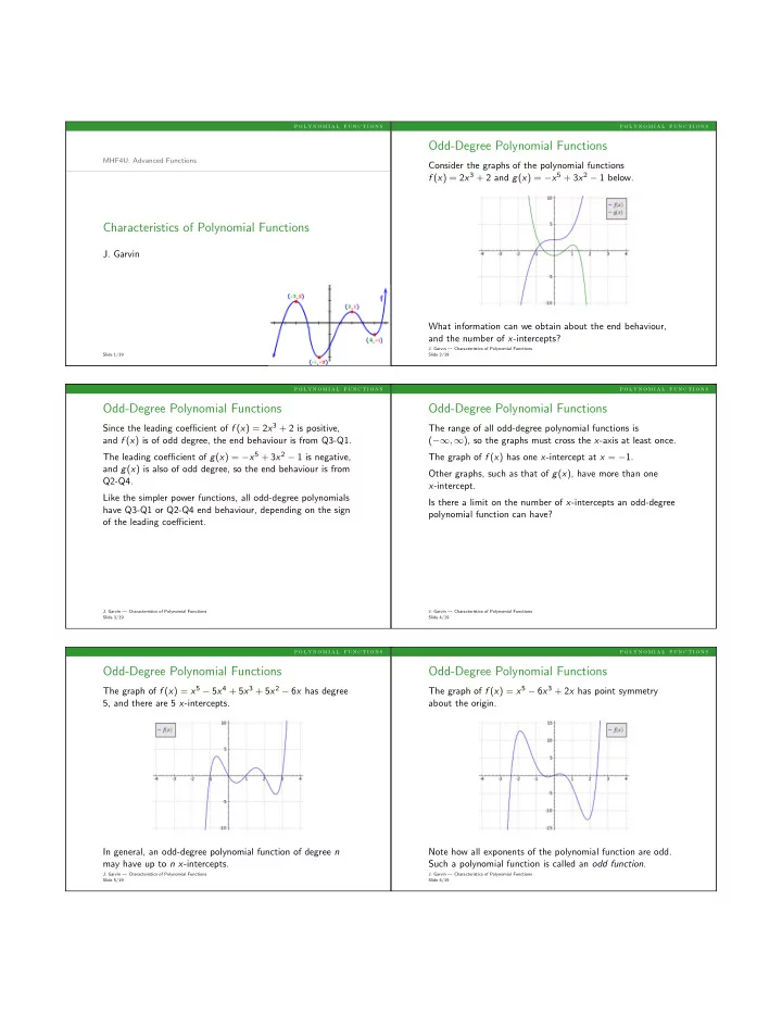
Consider the graphs of the polynomial functions f (x) = 2x3 + 2 and g(x) = −x5 + 3x2 − 1 below. What information can we obtain about the end behaviour, and the number of x-intercepts?

J. Garvin — Characteristics of Polynomial Functions

Slide 2/19

p o l y n o m i a l f u n c t i o n s

Odd-Degree Polynomial Functions

Since the leading coefficient of f (x) = 2x3 + 2 is positive, and f (x) is of odd degree, the end behaviour is from Q3-Q1. The leading coefficient of g(x) = −x5 + 3x2 − 1 is negative, and g(x) is also of odd degree, so the end behaviour is from Q2-Q4. Like the simpler power functions, all odd-degree polynomials have Q3-Q1 or Q2-Q4 end behaviour, depending on the sign

f the leading coefficient.
J. Garvin — Characteristics of Polynomial Functions

Slide 3/19

p o l y n o m i a l f u n c t i o n s

Odd-Degree Polynomial Functions

The range of all odd-degree polynomial functions is (−∞, ∞), so the graphs must cross the x-axis at least once. The graph of f (x) has one x-intercept at x = −1. Other graphs, such as that of g(x), have more than one x-intercept. Is there a limit on the number of x-intercepts an odd-degree polynomial function can have?

J. Garvin — Characteristics of Polynomial Functions

Slide 4/19

p o l y n o m i a l f u n c t i o n s

Odd-Degree Polynomial Functions

The graph of f (x) = x5 − 5x4 + 5x3 + 5x2 − 6x has degree 5, and there are 5 x-intercepts. In general, an odd-degree polynomial function of degree n may have up to n x-intercepts.

J. Garvin — Characteristics of Polynomial Functions

Slide 5/19

p o l y n o m i a l f u n c t i o n s

Odd-Degree Polynomial Functions

The graph of f (x) = x5 − 6x3 + 2x has point symmetry about the origin. Note how all exponents of the polynomial function are odd. Such a polynomial function is called an odd function.

J. Garvin — Characteristics of Polynomial Functions

Slide 6/19

SLIDE 2

p o l y n o m i a l f u n c t i o n s

Even-Degree Polynomial Functions

Consider the graphs of the polynomial functions f (x) = 3x2 + 1 and g(x) = −x4 + 6x2 − x − 4 below. Even-degree polynomial functions, such as f (x) and g(x), of degree n can have between 0 and n x-intercepts.

J. Garvin — Characteristics of Polynomial Functions

Slide 7/19

p o l y n o m i a l f u n c t i o n s

Even-Degree Polynomial Functions

Since the leading coefficient of f (x) = 3x2 + 1 is positive, the end behaviour is from Q2-Q1. The leading coefficient of g(x) = −x4 + 6x2 − x − 4 is negative, and the end behaviour is from Q3-Q4. Again, the end behaviour of even-degree polynomial functions is similar to power functions, and depends on the sign of the leading coefficient.

J. Garvin — Characteristics of Polynomial Functions

Slide 8/19

p o l y n o m i a l f u n c t i o n s

Even-Degree Polynomial Functions

The graph of f (x) = 3x4 − 2x2 − 3 is symmetric in the f (x)-axis. Note how all exponents of the polynomial function are even. Such a polynomial function is called an even function.

J. Garvin — Characteristics of Polynomial Functions

Slide 9/19

p o l y n o m i a l f u n c t i o n s

Classifying Polynomial Functions

Example

Classify f (x) as even, odd or neither. Although the function extends from Q3-Q4, it is not symmetric in the f (x)-axis, so it is neither even nor odd.

J. Garvin — Characteristics of Polynomial Functions

Slide 10/19

p o l y n o m i a l f u n c t i o n s

Classifying Polynomial Functions

Example

A polynomial function has x-intercepts at 0, 2, −3 and 7. What is the minimum degree of the polynomial if it is even? If it is odd? Since there are four distinct x-intercepts, the minimum degree of the polynomial is 4, in the case where the degree is even. If the function has odd degree, the minimum degree must be 5, since a cubic function (degree 3) can have at most 3 x-intercepts.

J. Garvin — Characteristics of Polynomial Functions

Slide 11/19

p o l y n o m i a l f u n c t i o n s

Finite Differences

Given a table of values for a polynomial function, it is possible to determine the value of the leading coefficient. First, let’s define n! (“n factorial”) as follows: n! = n × (n − 1) × (n − 2) × . . . × 2 × 1 Some examples: 3! = 3 × 2 × 1 = 6 10! = 10 × 9 × . . . × 2 × 1 = 3 628 800

J. Garvin — Characteristics of Polynomial Functions

Slide 12/19

SLIDE 3

p o l y n o m i a l f u n c t i o n s

Finite Differences

Let’s examine the finite differences for f (x) = x3. x f (x) ∆1 ∆2 ∆3 1 1 1 2 8 7 6 3 27 19 12 6 4 64 37 18 6 5 125 61 24 6 Note that f (x) has degree 3 and the third differences are constant. Also note that 3! = 6, which is the value of the third differences.

J. Garvin — Characteristics of Polynomial Functions

Slide 13/19

p o l y n o m i a l f u n c t i o n s

Finite Differences

Now let’s examine the finite differences for f (x) = −2x4. x f (x) ∆1 ∆2 ∆3 ∆4 1

2

3

4

5

1250
738
388
168
48

f (x) has degree 4 and the fourth differences are constant. 4! = 24, which is not the value of the fourth differences. However, multiplying 4! by the leading coefficient, −2, does produce the value −48.

J. Garvin — Characteristics of Polynomial Functions

Slide 14/19

p o l y n o m i a l f u n c t i o n s

Finite Differences

Finite Differences for Polynomial Functions

Given a polynomial function with degree n and leading coefficient a, the nth finite differences are constant, with a value of an!. We can use this relationship to determine the leading coefficient of any polynomial function, given enough points

n its graph.
J. Garvin — Characteristics of Polynomial Functions

Slide 15/19

p o l y n o m i a l f u n c t i o n s

Finite Differences

Example

A polynomial function has constant fifth differences with a value of −360. Determine the degree of the function, and its leading coefficient. Since the fifth differences are constant, the degree is 5. Rearranging a × 5! = −360 to solve for a, we obtain a = −360

5!

= −360

120 = −3.

J. Garvin — Characteristics of Polynomial Functions

Slide 16/19

p o l y n o m i a l f u n c t i o n s

Finite Differences

Example

Determine the leading coefficient of the cubic function below. Four successive points are (−1, −1),(0, 0),(1, 1) and (2, −4).

J. Garvin — Characteristics of Polynomial Functions

Slide 17/19

p o l y n o m i a l f u n c t i o n s

Finite Differences

Construct a table of finite differences. x f (x) ∆1 ∆2 ∆3

1 1 1 1 2

Rearranging a × 3! = −6 to solve for a, we obtain a = −6

3! = −6 6 = −1.

J. Garvin — Characteristics of Polynomial Functions

Slide 18/19

MHF4U: Advanced Functions

Characteristics of Polynomial Functions

Odd-Degree Polynomial Functions

Consider the graphs of the polynomial functions f (x) = 2x3 + 2 and g(x) = −x5 + 3x2 − 1 below. What information can we obtain about the end behaviour, and the number of x-intercepts?

Odd-Degree Polynomial Functions

Odd-Degree Polynomial Functions

Odd-Degree Polynomial Functions

The graph of f (x) = x5 − 5x4 + 5x3 + 5x2 − 6x has degree 5, and there are 5 x-intercepts. In general, an odd-degree polynomial function of degree n may have up to n x-intercepts.

Odd-Degree Polynomial Functions

The graph of f (x) = x5 − 6x3 + 2x has point symmetry about the origin. Note how all exponents of the polynomial function are odd. Such a polynomial function is called an odd function.

Even-Degree Polynomial Functions

Consider the graphs of the polynomial functions f (x) = 3x2 + 1 and g(x) = −x4 + 6x2 − x − 4 below. Even-degree polynomial functions, such as f (x) and g(x), of degree n can have between 0 and n x-intercepts.

Even-Degree Polynomial Functions

Even-Degree Polynomial Functions

The graph of f (x) = 3x4 − 2x2 − 3 is symmetric in the f (x)-axis. Note how all exponents of the polynomial function are even. Such a polynomial function is called an even function.

Classifying Polynomial Functions

Example

Classify f (x) as even, odd or neither. Although the function extends from Q3-Q4, it is not symmetric in the f (x)-axis, so it is neither even nor odd.

Classifying Polynomial Functions

Example

Finite Differences

Finite Differences

Let’s examine the finite differences for f (x) = x3. x f (x) ∆1 ∆2 ∆3 1 1 1 2 8 7 6 3 27 19 12 6 4 64 37 18 6 5 125 61 24 6 Note that f (x) has degree 3 and the third differences are constant. Also note that 3! = 6, which is the value of the third differences.

Finite Differences

Now let’s examine the finite differences for f (x) = −2x4. x f (x) ∆1 ∆2 ∆3 ∆4 1

2

3

4

5

f (x) has degree 4 and the fourth differences are constant. 4! = 24, which is not the value of the fourth differences. However, multiplying 4! by the leading coefficient, −2, does produce the value −48.

Finite Differences

Finite Differences for Polynomial Functions

Given a polynomial function with degree n and leading coefficient a, the nth finite differences are constant, with a value of an!. We can use this relationship to determine the leading coefficient of any polynomial function, given enough points

Finite Differences

Example

A polynomial function has constant fifth differences with a value of −360. Determine the degree of the function, and its leading coefficient. Since the fifth differences are constant, the degree is 5. Rearranging a × 5! = −360 to solve for a, we obtain a = −360

5!

= −360

120 = −3.

Finite Differences

Example

Determine the leading coefficient of the cubic function below. Four successive points are (−1, −1),(0, 0),(1, 1) and (2, −4).

Finite Differences

Construct a table of finite differences. x f (x) ∆1 ∆2 ∆3

1 1 1 1 2

Rearranging a × 3! = −6 to solve for a, we obtain a = −6

3! = −6 6 = −1.

Questions?