numerical simulations of viscoelastic flows in fibrous
play

NUMERICAL SIMULATIONS OF VISCOELASTIC FLOWS IN FIBROUS POROUS MEDIA - PDF document

18 TH INTERNATIONAL CONFERENCE ON COMPOSITE MATERIALS NUMERICAL SIMULATIONS OF VISCOELASTIC FLOWS IN FIBROUS POROUS MEDIA H. L. Liu and W. R. Hwang* School of Mechanical Engineering, Gyeongsang National University, Jinju, South Korea *


  1. 18 TH INTERNATIONAL CONFERENCE ON COMPOSITE MATERIALS NUMERICAL SIMULATIONS OF VISCOELASTIC FLOWS IN FIBROUS POROUS MEDIA H. L. Liu and W. R. Hwang* School of Mechanical Engineering, Gyeongsang National University, Jinju, South Korea * Corresponding author (wrhwang@gnu.ac.kr) Keywords : viscoelastic flow, porous media, flow resistance, resin transfer molding 1 Introduction on the flow resistance in various uni-directional Viscoelastic flow in porous media has important fibrous porous microstructures. applications in engineering fields such as composite manufacturing, textile coating and chemical 2 Modeling enhanced oil recovery industry. The flow resistance of polymeric surfactant in porous system is of great interest. Experimental results [1-4] indicate a gradually increment dramatic increase of flow resistance above a critical Weissenberg number. However, the steady state numerical simulations show that no evident increase of flow resistance with increasing pure elasticity [5-8]. Talwar and Khomami [9] simulated creeping flow of shear thinning viscoelastic fluids past periodic regular arrays of fibers with different viscoelastic models and their results indicated that as the pressure drop is progressively increased, the flow resistance 
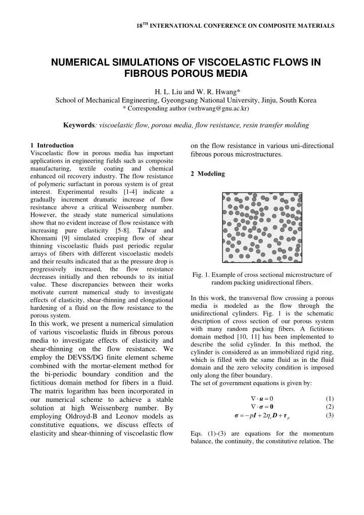
Fig. 1. Example of cross sectional microstructure of decreases initially and then rebounds to its initial random packing unidirectional fibers. value. These discrepancies between their works motivate current numerical study to investigate In this work, the transversal flow crossing a porous effects of elasticity, shear-thinning and elongational media is modeled as the flow through the hardening of a fluid on the flow resistance to the unidirectional cylinders. Fig. 1 is the schematic porous system. description of cross section of our porous system In this work, we present a numerical simulation with many random packing fibers. A fictitious of various viscoelastic fluids in fibrous porous domain method [10, 11] has been implemented to media to investigate effects of elasticity and describe the solid cylinder. In this method, the shear-thinning on the flow resistance. We cylinder is considered as an immobilized rigid ring, employ the DEVSS/DG finite element scheme which is filled with the same fluid as in the fluid combined with the mortar-element method for domain and the zero velocity condition is imposed the bi-periodic boundary condition and the only along the fiber boundary. fictitious domain method for fibers in a fluid. The set of government equations is given by: The matrix logarithm has been incorporated in ∇⋅ = u 0 (1) our numerical scheme to achieve a stable ∇⋅ = 0 σ (2) solution at high Weissenberg number. By = − + η + σ p I D τ 2 (3) employing Oldroyd-B and Leonov models as s p constitutive equations, we discuss effects of elasticity and shear-thinning of viscoelastic flow Eqs. (1)-(3) are equations for the momentum balance, the continuity, the constitutive relation. The

  2. formulation, we introduce an extra variable e , the constitutive relations of employed viscoelastic models are given as: viscous polymer stress. ∇ λ + − η = τ τ D 2 0, (4) p p p = η e D 2 (10) p ∇ 1 1 + − ⋅ = τ τ τ τ G D, 2 (5) p λ p λ p p G 2 We introduced three different Lagrangian multipliers ∂ τ ∇ ( ) B i T λ , λ h λ v ≡ p + ⋅∇ − ∇ ⋅ − ⋅∇ τ u τ u τ τ u. , and , which are associated with the rigid- (6) p ∂ p p p t − ring constraint along the i t h fiber, kinematic constrains for periodicity in horizontal and vertical Eqs. (4) and (5) are Oldroyd-B and Leonov models directions. The weak form for the whole domain can ∇ as constitutive equations and symbol ‘ ’ denotes be stated as: Find ( ) the upper-convected time derivative which is define u p τ e λ i λ λ B , h v such that , , , , , , p by Eq. (6). Following previous works [7-9], the [ ] [ ] [ ] ∫ ∫ ∫ − ∇⋅ Ω + η Ω − Ω p v d D v D u d e : D v d corrected flow resistance coefficient which only :2 0 Ω Ω Ω represents the effect of elasticity is the ratio of flow N ( ) ∑ λ + − rates in porous media between the corresponding i B, v λ v h y v L y ( , )+ , (0, ) ( , ) , Γ inelastic viscous and viscoelastic flows as: = i 4 1 ( ) [ ] ∫ + − = Ω λ v x H v x τ D v d v , ( , ) ( ,0) : , (11) p Q Γ Ω 3 = fRe viscous . (7) ∫ Ω ∇⋅ Ω = q v d corr . Q 0, (12) viscoelastic ( ) 1 ∫ ∫ − Ω + Ω = e D u d e e d : : 0, (13) The Carreau-Yasuda model, including a Newtonian s s η Ω Ω 2 p η , is employed to describe the solvent viscosity s ⎛ ⎞ ∇ ∫ S λ + − η Ω τ τ D d ⎜ ⎟ inelastic non-Newtonian flow as: : 2 p p p ⎝ ⎠ Ω nel η ( ) ( ∑ ∫ ) − λ − ⋅ Γ = S τ τ ext u n d η = η + : 0 , (14) 0 (8) p p ( ) cy s − n a 1 ⎡ ( ) ⎤ a = Γ + λγ e � 1 in 1 e ⎣ ⎦ B, , = = μ i u i N ( ) 0, ( 1,..., ) (15) ( ) − = μ u y u L y h , (0, ) ( , ) 0, (16) Furthermore, the Weissenberg number is defined by: Γ 4 ( ) − = μ u x H u x v , ( , ) ( ,0) 0, (17) = λ We Q L 2 (9) Γ 3 for all ( ) v q S e μ i μ μ B , h v . , , , , , , s where λ is the relaxation time of viscoelastic fluid , For the discretization of the weak form, we employ Q is the flow rate and L represents the the regular quadrilateral elements with continuous characteristic length of interstice in porous bi-quadratic interpolation for the velocity u , microstructure. discontinuous linear interpolation for the pressure p , continuous bi-linear interpolation for the viscous 4. Numerical methods polymer stress e and discontinuous bi-linear τ interpolation for the polymer stress . The polymer We employ the DEVSS scheme which is a mixed p finite-element method together with the Matrix stress tensor is treated by a matrix logarithmic Logarithms for accurate and stable computation of formulation and thus the stable solution to high viscoelastic flow to a relative high Weissenberg Weissenberg number has been achieved [12]. number. The DG formulation is used for the After implementing above discretization, one gets a discretization of the viscoelastic constitutive sparse matrix with non-zeros off the diagonal. A equation. For the combination of the DEVSS direct solver (HSL2002/MA41) based on the sparse

  3. PAPER TITLE multi-frontal variant of Gaussian elimination is used done by Skartsis et al. [2]. The numerically to solve the final matrix. determined flow resistance is presented as a function of Weissenberg number in Fig. 3. The previous numerical results by UCM and Oldroyd-B models 3 Results and discussion have also been reproduced along with our results. The experiment data manifest a dramatic increase of We performed the mesh refinement test for the flow resistance above a critical Weissenberg number Oldroyd-B fluid with a cylinder in the center of a ( ) We = square domain. The radius of the fiber is 0.2 and the 0.25 , however the numerical predictions by size of domain is 1×1. We used three different Talwar and Khomami [8] for both models indicate a meshes of 25×25, 50×50 and 100×100 elements, steady decline of fluid resistance with the restriction which are denoted by M1, M2 and M3, respectively. We = to Weissenberg number at about 5 . In contrast The trace of conformation tensor along the center to their numerical results, our computation show a ( ) x = line 0.5 under three different meshes M1, M2 We = slight increase of flow resistance until 20 . and M3 are presented in Fig. 2 and indicate good convergence in the mesh refinement. In addition, we checked the introduction of the matrix logarithm and the result shows that the implement of matrix logarithm eliminates the instable oscillation around the interface between the fiber and viscoelastic fluid. Fig. 3. The flow resistance predictions by Oldroyed- B model in a square packing fiber array with the comparison with earlier experimental data [2] and numerical study [8]. In order to understand the effect of fiber configuration on flow resistance, we performance the flow simulation by both Oldroyd-B and Leonov Fig. 2. The mesh convergence test for the Oldroyd-B models in 100 random packing fibers as depicted in fluid past a cylinder with three different meshes, as Fig. 1. The numerical predicted flow resistance in well as the comparison with the implement of the 100 random packing fibers shows a dramatic matrix logarithm. increase of flow resistance with respect to Weissenberg number by Oldroyed-B model as Having validated our numerical scheme, we plotted in Fig. 4. Furthermore, the corrected friction compare our simulation of Oldroyd-B fluid with coefficient for Leonov model, which only reflect the previous experimental and numerical studies for the elasticity effects on flow resistance by exclusion the problem involved flows of Boger fluids through shear thinning effect, also exhibits the steady square array of motionless cylinders [2, 8]. The increase. For the case of square packing fibers, the simulation conditions are fitted to the experiments 3

Download Presentation
Download Policy: The content available on the website is offered to you 'AS IS' for your personal information and use only. It cannot be commercialized, licensed, or distributed on other websites without prior consent from the author. To download a presentation, simply click this link. If you encounter any difficulties during the download process, it's possible that the publisher has removed the file from their server.

Recommend


More recommend