NUMERICAL SIMULATION OF THE RTM LIGHT MANUFACTURING PROCESS J. Timms - - PDF document

18TH INTERNATIONAL CONFERENCE ON COMPOSITE MATERIALS

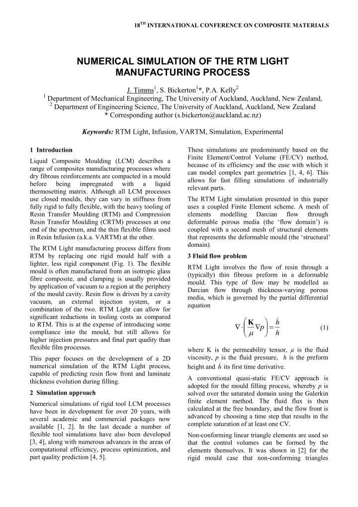
1 Introduction Liquid Composite Moulding (LCM) describes a range of composites manufacturing processes where dry fibrous reinforcements are compacted in a mould before being impregnated with a liquid thermosetting matrix. Although all LCM processes use closed moulds, they can vary in stiffness from fully rigid to fully flexible, with the heavy tooling of Resin Transfer Moulding (RTM) and Compression Resin Transfer Moulding (CRTM) processes at one end of the spectrum, and the thin flexible films used in Resin Infusion (a.k.a. VARTM) at the other. The RTM Light manufacturing process differs from RTM by replacing one rigid mould half with a lighter, less rigid component (Fig. 1). The flexible mould is often manufactured from an isotropic glass fibre composite, and clamping is usually provided by application of vacuum to a region at the periphery

• f the mould cavity. Resin flow is driven by a cavity

vacuum, an external injection system, or a combination of the two. RTM Light can allow for significant reductions in tooling costs as compared to RTM. This is at the expense of introducing some compliance into the mould, but still allows for higher injection pressures and final part quality than flexible film processes. This paper focuses on the development of a 2D numerical simulation of the RTM Light process, capable of predicting resin flow front and laminate thickness evolution during filling. 2 Simulation approach Numerical simulations of rigid tool LCM processes have been in development for over 20 years, with several academic and commercial packages now available [1, 2]. In the last decade a number of flexible tool simulations have also been developed [3, 4], along with numerous advances in the areas of computational efficiency, process optimization, and part quality prediction [4, 5]. These simulations are predominantly based on the Finite Element/Control Volume (FE/CV) method, because of its efficiency and the ease with which it can model complex part geometries [1, 4, 6]. This allows for fast filling simulations of industrially relevant parts. The RTM Light simulation presented in this paper uses a coupled Finite Element scheme. A mesh of elements modelling Darcian flow through deformable porous media (the ‘flow domain’) is coupled with a second mesh of structural elements that represents the deformable mould (the ‘structural’ domain). 3 Fluid flow problem RTM Light involves the flow of resin through a (typically) thin fibrous preform in a deformable

• mould. This type of flow may be modelled as

Darcian flow through thickness-varying porous media, which is governed by the partial differential equation

h h p               K

(1) where K is the permeability tensor, µ is the fluid viscosity, p is the fluid pressure, h is the preform height and h  its first time derivative. A conventional quasi-static FE/CV approach is adopted for the mould filling process, whereby p is solved over the saturated domain using the Galerkin finite element method. The fluid flux is then calculated at the free boundary, and the flow front is advanced by choosing a time step that results in the complete saturation of at least one CV. Non-conforming linear triangle elements are used so that the control volumes can be formed by the elements themselves. It was shown in [2] for the rigid mould case that non-conforming triangles

NUMERICAL SIMULATION OF THE RTM LIGHT MANUFACTURING PROCESS

• J. Timms1, S. Bickerton1*, P.A. Kelly2

1 Department of Mechanical Engineering, The University of Auckland, Auckland, New Zealand, 2 Department of Engineering Science, The University of Auckland, Auckland, New Zealand

* Corresponding author (s.bickerton@auckland.ac.nz) Keywords: RTM Light, Infusion, VARTM, Simulation, Experimental

conserve fluid mass both within and between

• elements. However, this does not hold in general for

thickness varying elements, so a modification to the fluid flux qa proposed by Kelly [7] has been adopted:

   

B FE a

h h p x x K x q       2  

(2) where xB is the barycentre of the element. Equation 2 ensures intra-element mass conservation and, in the case of constant or linearly varying forcing terms, flux continuity between elements. Height is treated as constant across an element in this simulation, so the condition holds. Flow into unsaturated elements adjacent to the front boundary can be then be found by integrating the normal component of the linearly varying flux across the element edge. This allows for improved estimates of flow front progression without resorting to more computationally expensive mixed-methods. The current simulation is restricted to planar geometries, but this is sufficient to capture the majority of key behaviour, and the extension to 2.5D shell geometries is relatively straightforward. 4 Structural problem RTM Light mould compliance can potentially vary from near-rigid to very flexible due to differences in mould construction (e.g. material, thickness, use of stiffeners, etc.), part size, target volume fractions, and injection pressures. This paper considers the canonical RTM Light process, which has a rigid A- side mould, and a thin B-side mould constructed from a linearly elastic material. For planar geometries, the structural behaviour of this type of mould can be modelled by the Kirchhoff thin plate

• theory. This model requires that 1) the plate’s

thickness is small relative to its characteristic length, and 2) the deflections are small relative to the

• thickness. Both these conditions can be met by

requiring the B-side mould to be constructed from a sufficiently stiff material. In the case of isotropic, homogenous plates with a constant flexural rigidity D, deflection u is related to lateral distributed load b by

D b u  4

(3) Analytical solutions to Eq. 3 exist for simple geometries and loading and boundary conditions. along with Green’s functions for deflection for general loading states [8]. However, a useful RTM Light simulation requires deflection of non-regular mould geometries, as well as an ability to handle more advanced construction features, such as anisotropic materials, variable thickness, and the application of stiffeners. For these reasons, it is necessary to adopt a numerical solution procedure. While a number of alternative numerical procedures are available for thin plate problems, such as the boundary element method, the finite element method is preferred in this simulation because of its numerical efficiency, established literature, and

• versatility. It is easily extended into 2.5D by

adopting shell elements, and to thick plates by using those based on Reissner-Mindlin thick plate theory

• r 3D elasticity. Furthermore, many of the assembly

and solver routines can be shared between the flow and structural finite element modules. The plate bending element is the 9 DOF discrete Kirchhoff triangle (DKT), implemented using the local coordinate formulation given by Batoz [9]. While faster converging elements are available, the DKT is suitable for this simulation because of its reliability and low numerical overhead. Clamped, simple support, and free edge boundary conditions can be specified. In the current simulation, the same mesh is used for the structural and flow problems. Deflections and loads are lumped in a consistent manner and passed between solvers during each iteration. 6 Coupling and solution procedure The flow equation (Eq. 1) is coupled to the structural problem by the dependence of height and permeability on mould displacement u:

 

t h K K , ,x 

(4)

   

x x , h t u h  

(5) where h0 is a reference height at zero deflection. Similarly, the structural problem is coupled to the flow problem by the dependence of the lateral load q

• n the resin pressure:

 

p p b

f ext

   

(6)

3 NUMERICAL SIMULATION OF THE RTM LIGHT MANUFACTURING PROCESS

where pext is the external loading (typically atmospheric pressure), σf is the fibre compaction stress and p is the resin pressure. The iterative solution procedure used to solve the system is flowcharted in Fig. 3. The first stage is to determine the initial mould deflection for the dry preform, i.e. with a zero fluid pressure loading term:

 

h u p b

f ext

   

(7) Once determined, the filling stage coupling algorithm begins by guessing h , either by taking h  from the previous time step or a linear interpolation

• f the previous two time steps. The guess value is

passed to the flow module, and the fluid pressure, flux, and time step are calculated. The pressure is combined with the fibre compaction stress to determine the distributed load on the mould, which is then passed to the structural module. The calculated height profile and time step are used to updateh  using a backward difference discretisation. If the change in h  is within tolerance, the flow front is updated and time is advanced; otherwise, the guess value of h is updated. Initially the updated guess value was taken directly from the structural module result. However, this was found to produce large oscillations in the calculated pressure field. To reduce these oscillations, a weighting parameter ω was introduced, such that the updated guess was a weighted average of the calculated height and the previous guess:

 

1 1

1

 

  

i t i t i t

h h h     

(8) 7 Numerical Studies A series of numerical experiments have been conducted to test the efficacy of the simulation. Rates of convergence for the current coupling algorithm are slow, particularly for large mould deflections ( >10% initial cavity height), and faster convergence is only available at the expense of

• stability. The cases presented here therefore only

cover high rigidity moulds with small deflections. Despite this, the effects of mould compliance on LCM mould filling can still be observed. Both cases are based on a 1 m x 1 m square mould, with a cavity height of 4.25 mm. The reinforcement parameters are based on an isotropic E-glass chopped strand mat (CSM). Compaction and permeability relations are based on experimental data presented by Walbran in [10]. For the permeability an exponential model is used:

 

2 8

m 97 . 12 exp 10 07 . 3

f ii

V K   



(8) and the compaction response is modelled with a fourth order polynomial: Pa 10 . 3 10 6 . 3 10 7 . 1 10 7 . 3 10 9 . 2

4 7 3 7 2 7 6 5 f f f f f

V V V V            (9) Other parameters are listed in Table 1. All studies used a constant pressure injection scheme, with no

• vacuum. This is equivalent to setting pext = 0. For

each case four different upper mould thickness were considered: 35mm, 50mm, 75mm, and 100mm. The material properties for the upper mould were those

• f structural steel, with a Young’s modulus of 200

GPa and a Poisson’s ratio of 0.3. The mould thicknesses are at the upper end of the acceptable range for applying Kirchhoff plate theory, but this is not particularly crucial for these expository studies. A clamped boundary condition is applied to the mould edge. 7.1 Case 1: Rectilinear filling of a square mould The first case considers rectilinear filling, with a line gate and vent along opposing sides. A 4096 element mesh right sided triangles was used. Only half the mould was meshed, with symmetry conditions for the plate and structural domain being applied to the centreline edge. Fig. 4 shows the mould cavity thickness for the 35 mm upper mould at the completion of filling. The peak deflection occurs at (0.5,0.45) – slightly behind the centre point of the mould – due to the fluid pressure gradient. The symmetry line cavity thicknesses at the end of filling for all moulds are shown in Fig. 5. Peak deflections range from 8.23% to 0.4% of h0. These thickness changes have little effect in the corresponding fluid pressures, as can be seen in Fig.

• 6. The small difference is likely due to the relatively

small changes in permeability and porous volumes, even for the 35 mm mould. Fill time as a function of normalised flexural rigidity is presented in Fig. 7. The fill time appears to converge towards the rigid (RTM) value as expected, but the convergence is from above, not from below

as would be expected with decreasing volume fraction and permeability. This may be a consequence of the true differences in fill time being within the approximation error of the flow front

• predictions. Further investigation into this behaviour

is necessary. 7.2 Case 2: Radial filling of a square mould The radial filling case – central injection with a perimeter gate – was analysed with a 2048 element quarter-square mesh of right sided triangles. Symmetry boundary conditions were applied on the left and bottom edges. Fig. 8 shows the mould deflections for the 35 mm mould at the end of filling across the entire mesh, and the end of filling deflection along a 45° line from the inlet is presented in Fig. 9 for each mould. The fluid pressure at the same points is given in Fig. 10 Compared with the rectilinear case, there is a larger difference in the fluid pressure profile as mould stiffness changes (Fig. 11). The direction of this change is consistent with experimentally observed data for axisymmetric RTM Light processes [11]. The behaviour of fill time with mould rigidity is more consistent with expectations for the radial filling case (Fig. 11), with fill times converging towards the rigid mould value from below. The sensitivity of fill time is much higher for the radial case, with fill times up to 14% faster than rigid mould case, compared to 2% difference for the same mould in rectilinear filling. This is likely due to the concentration of high fluid pressure near the center

• f the mould, resulting in larger bending moments

and greater deflections. The greatest pressure drop

• ccurs in this region, so the deflection and its effect
• n permeability have a maginified effect.

8 Conclusions and future work A 2D simulation of the RTM Light composites manufacturing process has been described. It couples a finite element/control volume simulation fluid flow in deformable porous media with a plate- bending finite element solver, using elements based

• n the Kirchhoff thin plate theory. Results have been

shown for two case studies – rectilinear and radial flow in a square mould. The simulation is showing qualitatively good results at low deflections, but numerical stability and convergence issues remain at larger deflections. Further development in this area is in progress, along with other improvements, such as the incorporation of the post-filling resin bleeding stage, extension to 2.5D shell structures, and experimental validation.

Table 1: Process parameters for case studies

Datum height, h0 4.25 mm Datum volume fraction, Vf0 0.410 Fluid viscosity 0.5 Pa.s Injection pressure 5 bar Vent pressure 1 bar

• Fig. 1 Schematic of the RTM Light manufacturing

process.

• Fig. 2 Coupling algorithm flowchart

as would be expected with decreasing volume fraction and permeability. This may be a consequence of the true differences in fill time being within the approximation error of the flow front

• predictions. Further investigation into this behaviour

is necessary. 7.2 Case 2: Radial filling of a square mould The radial filling case – central injection with a perimeter gate – was analysed with a 2048 element quarter-square mesh of right sided triangles. Symmetry boundary conditions were applied on the left and bottom edges. Fig. 8 shows the mould deflections for the 35 mm mould at the end of filling across the entire mesh, and the end of filling deflection along a 45° line from the inlet is presented in Fig. 9 for each mould. The fluid pressure at the same points is given in Fig. 10 Compared with the rectilinear case, there is a larger difference in the fluid pressure profile as mould stiffness changes (Fig. 11). The direction of this change is consistent with experimentally observed data for axisymmetric RTM Light processes [11]. The behaviour of fill time with mould rigidity is more consistent with expectations for the radial filling case (Fig. 11), with fill times converging towards the rigid mould value from below. The sensitivity of fill time is much higher for the radial case, with fill times up to 14% faster than rigid mould case, compared to 2% difference for the same mould in rectilinear filling. This is likely due to the concentration of high fluid pressure near the center

• f the mould, resulting in larger bending moments

and greater deflections. The greatest pressure drop

• ccurs in this region, so the deflection and its effect
• n permeability have a maginified effect.

8 Conclusions and future work A 2D simulation of the RTM Light composites manufacturing process has been described. It couples a finite element/control volume simulation fluid flow in deformable porous media with a plate- bending finite element solver, using elements based

• n the Kirchhoff thin plate theory. Results have been

shown for two case studies – rectilinear and radial flow in a square mould. The simulation is showing qualitatively good results at low deflections, but numerical stability and convergence issues remain at larger deflections. Further development in this area is in progress, along with other improvements, such as the incorporation of the post-filling resin bleeding stage, extension to 2.5D shell structures, and experimental validation.

Table 1: Process parameters for case studies

Datum height, h0 4.25 mm Datum volume fraction, Vf0 0.410 Fluid viscosity 0.5 Pa.s Injection pressure 5 bar Vent pressure 1 bar

• Fig. 1 Schematic of the RTM Light manufacturing

process.

• Fig. 2 Coupling algorithm flowchart

Preform Assembly and Placement Pre-Filling Compaction and Debulking Resin Injection Post-Filling Thickness Consolidation

as would be expected with decreasing volume fraction and permeability. This may be a consequence of the true differences in fill time being within the approximation error of the flow front

• predictions. Further investigation into this behaviour

is necessary. 7.2 Case 2: Radial filling of a square mould The radial filling case – central injection with a perimeter gate – was analysed with a 2048 element quarter-square mesh of right sided triangles. Symmetry boundary conditions were applied on the left and bottom edges. Fig. 8 shows the mould deflections for the 35 mm mould at the end of filling across the entire mesh, and the end of filling deflection along a 45° line from the inlet is presented in Fig. 9 for each mould. The fluid pressure at the same points is given in Fig. 10 Compared with the rectilinear case, there is a larger difference in the fluid pressure profile as mould stiffness changes (Fig. 11). The direction of this change is consistent with experimentally observed data for axisymmetric RTM Light processes [11]. The behaviour of fill time with mould rigidity is more consistent with expectations for the radial filling case (Fig. 11), with fill times converging towards the rigid mould value from below. The sensitivity of fill time is much higher for the radial case, with fill times up to 14% faster than rigid mould case, compared to 2% difference for the same mould in rectilinear filling. This is likely due to the concentration of high fluid pressure near the center

• f the mould, resulting in larger bending moments

and greater deflections. The greatest pressure drop

• ccurs in this region, so the deflection and its effect
• n permeability have a maginified effect.

8 Conclusions and future work A 2D simulation of the RTM Light composites manufacturing process has been described. It couples a finite element/control volume simulation fluid flow in deformable porous media with a plate- bending finite element solver, using elements based

• n the Kirchhoff thin plate theory. Results have been

shown for two case studies – rectilinear and radial flow in a square mould. The simulation is showing qualitatively good results at low deflections, but numerical stability and convergence issues remain at larger deflections. Further development in this area is in progress, along with other improvements, such as the incorporation of the post-filling resin bleeding stage, extension to 2.5D shell structures, and experimental validation.

Table 1: Process parameters for case studies

Datum height, h0 4.25 mm Datum volume fraction, Vf0 0.410 Fluid viscosity 0.5 Pa.s Injection pressure 5 bar Vent pressure 1 bar

• Fig. 1 Schematic of the RTM Light manufacturing

process.

• Fig. 2 Coupling algorithm flowchart

Preform Assembly and Placement Pre-Filling Compaction and Debulking Resin Injection Post-Filling Thickness Consolidation

5 NUMERICAL SIMULATION OF THE RTM LIGHT MANUFACTURING PROCESS

• Fig. 3 Mould cavity thickness in mm at the end of filling.

35 mm upper mould. Rectilinear filling.

• Fig. 4 Mould cavity thickness at the end of filling along

the center line (x=0.5) for a range of upper moulds. Rectilinear filling.

• Fig. 5 Fluid pressure at the end of filling along the center

line (x=0.5) for a range of upper moulds. Rectilinear filling

• Fig. 6 Deviation in fill time as a function of mould

flexural rigidity. Rectilinear filling.

• Fig. 7 Mould cavity thickness in mm at the end of filling.

35 mm upper mould. Radial filling.

• Fig. 8 Mould cavity thickness at the end of filling for a

range of upper moulds. Radial filling.Samples are taken along the 45° line. x (m) y (m) 0.25 0.5 0.25 0.5 0.75 1 4.2 4.3 4.4 4.5

0.25 0.5 0.75 1 4.2 4.3 4.4 4.5 4.6 4.7 4.7 Distance from inlet (m) Cavity thickness (mm) 100 mm 75 mm 50 mm 35 mm

0.25 0.5 0.75 1 100 200 300 400 Distance from inlet (m) Fluid pressure (kPa) 100 mm 75 mm 50 mm 35 mm

0.25 0.5 0.75 1 0.5 1 1.5 2 2.5 Relative mould flexural rigidty (D/Dmax) % deviation from RTM (rigid) fill time

x (m) y (m) 0.25 0.5 0.25 0.5 4.2 4.3 4.4 4.5 0.1 0.2 0.3 0.4 0.5 4.2 4.3 4.4 4.5 Distance from inlet (m) Cavity thickness (mm) 100 mm 75 mm 50 mm 35 mm

sampling line

• Fig. 9 Fluid pressure at the end of filling for a range of

upper moulds. Radial filling.

• Fig. 10 Deviation in fill time as a function of mould

flexural rigidity. Radial filling.

References

[1] M.V. Bruschke and S.G. Advani "A finite element/control volume approach to mold filling in anisotropic porous media". Polymer Composites,

• Vol. 11, No. 6, pp 398-405, 1990.

[2]

• F. Trochu, R. Gauvin and D.M. Gao "Numerical

analysis of the resin transfer molding process by the finite element method". Advances in Polymer Technology, Vol. 12, No. 4, pp 329-42, 1993. [3]

• Q. Govignon, S. Bickerton and P.A. Kelly

"Simulation of the reinforcement compaction and resin flow during the complete resin infusion process". Composites Part A: Applied Science and Manufacturing, Vol. 41, No. 1, pp 45-57, 2010. [4]

• P. Simacek and S.G. Advani "Desirable features in

mold filling simulations for liquid composite molding processes". Polymer Composites, Vol. 25,

• No. 4, pp 355-67, 2004.

[5]

• F. Trochu, E. Ruiz, V. Achim and S. Soukane

"Advanced numerical simulation of liquid composite molding for process analysis and optimization". Composites Part A: Applied Science and Manufacturing, Vol. 37, No. 6, pp 890-902, 2006. [6] P.A. Kelly and S. Bickerton "A comprehensive filling and tooling force analysis for rigid mould LCM processes". Composites Part A: Applied Science and Manufacturing, Vol. 40, No. 11, pp 1685-97, 2009. [7] P.A. Kelly and S. Jennings "Nonconforming Elements for Liquid Composite Molding Process Simulation". Proceedings of 8th International Conference on Flow Processes in Composite Materials, Douai, France, 2006. [8] Y.A. Melnikov "Green's function of a thin circular plate with elastically supported edge". Engineering Analysis with Boundary Elements, Vol. 25, No. 8, pp 669-76, 2001. [9] J.L. Batoz, K.J. Bathe and L.W. Ho "Study of three- node triangular plate-bending elements.". International Journal for Numerical Methods in Engineering, Vol. 15, No. 12, pp 1771-812, 1980. [10] W.A. Walbran, B. Verleye, S. Bickerton and P.A. Kelly "Prediction and experimental verification of Normal Stress Distributions on Mould Tools During Liquid Composite Moulding". Composites Part A: Applied Science and Manufacturing, Vol. (In Press),

• No. pp 2011.

[11] J. Timms, Q. Govignon, S. Bickerton and P.A. Kelly "Observations from the filling and post-filling stages

• f axisymmetric liquid composite moulding with

flexible tooling". Proceedings of FPCM 10, Ascona, 2010.

0.1 0.2 0.3 0.4 0.5 100 200 300 400 Distance from inlet (m) Fluid pressure (kPa) 100 mm 75 mm 50 mm 35 mm 0.25 0.5 0.75 1

• 15
• 10
• 5

Relative mould flexural rigidty (D/Dmax) % deviation from RTM (rigid) fill time