Nonrecursive Model for Peer-Influences Data Variables in the Model - - PowerPoint PPT Presentation

The R Statistical Computing Environment Basics and Beyond Structural Equation Models with the sem package

John Fox

McMaster University

ICPSR/Berkeley 2016

John Fox (McMaster University) Structural Equation Models ICPSR/Berkeley 2016 1 / 26

Nonrecursive Model for Peer-Influences Data

Variables in the Model

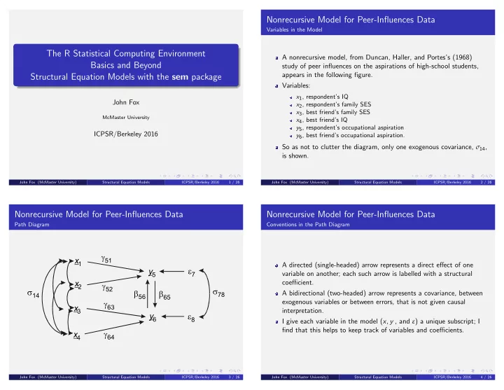
A nonrecursive model, from Duncan, Haller, and Portes’s (1968) study of peer influences on the aspirations of high-school students, appears in the following figure. Variables:

x1, respondent’s IQ x2, respondent’s family SES x3, best friend’s family SES x4, best friend’s IQ y5, respondent’s occupational aspiration y6, best friend’s occupational aspiration.

So as not to clutter the diagram, only one exogenous covariance, σ14, is shown.

John Fox (McMaster University) Structural Equation Models ICPSR/Berkeley 2016 2 / 26

Nonrecursive Model for Peer-Influences Data

Path Diagram

x1 x2 x3 x4 y5 y6 e7 e8 s78 s14 g51 g52 g63 g64 b56 b65

John Fox (McMaster University) Structural Equation Models ICPSR/Berkeley 2016 3 / 26

Nonrecursive Model for Peer-Influences Data

Conventions in the Path Diagram

A directed (single-headed) arrow represents a direct effect of one variable on another; each such arrow is labelled with a structural coefficient. A bidirectional (two-headed) arrow represents a covariance, between exogenous variables or between errors, that is not given causal interpretation. I give each variable in the model (x, y , and ε) a unique subscript; I find that this helps to keep track of variables and coefficients.

John Fox (McMaster University) Structural Equation Models ICPSR/Berkeley 2016 4 / 26

Nonrecursive Model for Peer-Influences Data

Structural Equations

The structural equations of a model can be read straightforwardly from the path diagram. For the Duncan, Haller, and Portes peer-influences model: y5i = γ50 + γ51x1i + γ52x2i + β56y6i + ε7i y6i = γ60 + γ63x3i + γ64x4i + β65y5i + ε8i

John Fox (McMaster University) Structural Equation Models ICPSR/Berkeley 2016 5 / 26

Nonrecursive Model for Peer-Influences Data

Structural Equations

I’ll usually simplify the structural equations by

1

suppressing the subscript i for observation;

2

expressing all xs and y s as deviations from their populations means (and, later, from their means in the sample).

Putting variables in mean-deviation form gets rid of the constant terms (here, γ50 and γ60) from the structural equations (which are rarely of interest), and will simplify some algebra later on. Applying these simplifications to the peer-influences model: y5 = γ51x1 + γ52x2 + β56y6 + ε7 y6 = γ63x3 + γ64x4 + β65y5 + ε8

John Fox (McMaster University) Structural Equation Models ICPSR/Berkeley 2016 6 / 26

Nonrecursive Model for Peer-Influences Data

Estimation Using the sem Package in R

The tsls function in the sem package is used to estimate structural equations by 2SLS. The function works much like the lm function for fitting linear models by OLS, except that instrumental variables are specified in the instruments argument as a “one-sided” formula. For example, to fit the first equation in the Duncan, Haller, and Portes model, we would specify something like eqn.1 <- tsls(ROccAsp ~ RIQ + RSES + FOccAsp, instruments= ~ RIQ + RSES + FSES + FIQ, data=DHP) summary(eqn.1) This assumes that we have Duncan, Haller, and Portes’s data in the data frame DHP, which is not the case. tsls can also perform weighted 2SLS estimation.

John Fox (McMaster University) Structural Equation Models ICPSR/Berkeley 2016 7 / 26

Nonrecursive Model for Peer-Influences Data

Estimation Using the sem Package in R

The sem function may be used to fit a wide variety of models — including observed-variable nonrecursive models — by FIML. The “data” for the model may be specified either in the form of a covariance matrix (or raw-moment matrix) or as case-by-variable data in the form of an R data frame; in either case, the first argument to sem is a description of the model to be fit. For moment-matrix input, there are three required arguments:

model: A coded formulation of the model, described below. S: The covariance matrix (or raw-moment matrix) among the observed variables in the model; may be in upper- or lower-triangular form as well as the full, symmetric matrix. N: The number of observations on which the moment matrix is based. In addition, for an observed-variable model, the argument fixed.x should be set to the names of the exogenous variables in the model.

John Fox (McMaster University) Structural Equation Models ICPSR/Berkeley 2016 8 / 26

Nonrecursive Model for Peer-Influences Data

Estimation Using the sem Package in R

If the original data set is available it is generally advantageous to use it; for example, it is then possible to obtain robust estimates of coefficient standard errors. For data-set input, there are two required arguments:

model: As before. data: An R data frame containing the data from which the covariance

• r raw moment matrix of the observed variables is computed.

In addition to fixed.x, there are two other arguments that are often useful:

formula: A one-sided R “model formula” to be applied to data to produce a numeric data matrix from which moments are computed; the default is ~. . raw: If TRUE (the default depends upon context but is typically FALSE), a raw-moment matrix is used rather than a covariance matrix, permitting the estimation of regression intercepts.

Additional arguments are available.

John Fox (McMaster University) Structural Equation Models ICPSR/Berkeley 2016 9 / 26

Nonrecursive Model for Peer-Influences Data

Estimation Using the sem Package in R

Internally, sem represents the model using a format called the “recticular-action model” (or RAM), which stems from an approach, due originally to McArdle, to specifying and estimating SEMs. The RAM model can be specified directly using the specifyModel function in the sem package, which returns a model-specification

• bject to be used as the first argument to sem:

Each structural coefficient of the model is represented as a directed arrow ->. Each error variance and covariance is represented as a bidirectional arrow, <->, linking an endogenous variables to itself or two endogenous variables, though specifyModel will by default supply error variances automatically for the endogenous variables in the model if these aren’t given explicitly.

To write out the model in the form required by specifyModel, it helps to redraw the path diagram, as in the following figure.

John Fox (McMaster University) Structural Equation Models ICPSR/Berkeley 2016 10 / 26

Nonrecursive Model for Peer-Influences Data

Modified path diagram omitting covariances among exogenous variables, and showing error variances and covariances as double arrows attached to the endogenous variables.

RIQ RSES FIQ FSES ROccAsp FOccasp gamma51 gamma63 gamma64 beta65 beta56 sigma88 sigma77 sigma78

John Fox (McMaster University) Structural Equation Models ICPSR/Berkeley 2016 11 / 26

Nonrecursive Model for Peer-Influences Data

Estimation Using the sem Package in R

Then the model can be encoded as follows, specifying each arrow, and giving a name to and start-value for the corresponding parameter (NA = let the program compute the start-value): model.DHP.1 <- specifyModel() RIQ

• >

ROccAsp, gamma51, NA RSES

• >

ROccAsp, gamma52, NA FSES

• >

FOccAsp, gamma63, NA FIQ

• >

FOccAsp, gamma64, NA FOccAsp -> ROccAsp, beta56, NA ROccAsp -> FOccAsp, beta65, NA ROccAsp <-> ROccAsp, sigma77, NA FOccAsp <-> FOccAsp, sigma88, NA ROccAsp <-> FOccAsp, sigma78, NA

John Fox (McMaster University) Structural Equation Models ICPSR/Berkeley 2016 12 / 26

Nonrecursive Model for Peer-Influences Data

Estimation Using the sem Package in R

As mentioned, the error-variance parameters need not be given directly, and one can also omit the NAs for the start values, and so a more compact equivalent specification would be model.DHP.1 <- specifyModel() RIQ

• >

ROccAsp, gamma51 RSES

• >

ROccAsp, gamma52 FSES

• >

FOccAsp, gamma63 FIQ

• >

FOccAsp, gamma64 FOccAsp -> ROccAsp, beta56 ROccAsp -> FOccAsp, beta65 ROccAsp <-> FOccAsp, sigma78

John Fox (McMaster University) Structural Equation Models ICPSR/Berkeley 2016 13 / 26

Nonrecursive Model for Peer-Influences Data

Estimation Using the sem Package in R

The specifyEquations function is often a more convenient and compact way to specify a structural equation model; for the current example: model.DHP.1 <- specifyEquations() ROccAsp = gamma51*RIQ + gamma52*RSES + beta56*FOccAsp FOccAsp = gamma64*FIQ + gamma63*FSES + beta65*ROccAsp C(ROccAsp, FOccAsp) = sigma78 Each term on the RHS of a structural equation is given in the form coefficient*explanatoryVariable. Error covariances are specified using C().

John Fox (McMaster University) Structural Equation Models ICPSR/Berkeley 2016 14 / 26

Nonrecursive Model for Peer-Influences Data

Estimation Using the sem Package in R

Error variances can be specified similarly using V(), but this is unnecessary here since specifyEquations supplies them by default. Parameter start values can optionally be given in parentheses after the parameter name; e.g., beta56(0.5)*FOccAsp. Fixed parameters can be specified using numeric constants; e.g. (not pertaining to the Duncan, Haller, and Portes data), 1*age.

John Fox (McMaster University) Structural Equation Models ICPSR/Berkeley 2016 15 / 26

Nonrecursive Model for Peer-Influences Data

Estimation Using the sem Package in R

As was common when SEMs were first introduced to sociologists, Duncan, Haller, and Porter estimated their model for standardized variables. That is, the covariance matrix among the observed variables is a correlation matrix. The arguments for using standardized variables in a SEM are no more compelling than in a regression model. In particular, it makes no sense to standardize dummy regressors, for example.

John Fox (McMaster University) Structural Equation Models ICPSR/Berkeley 2016 16 / 26

A Latent-Variable Model for the Peer-Influences Data

Path Diagram

x =

1 1

x x =

2 2

x x =

3 3

x x =

4 4

x x =

5 5

x x =

6 6

x s f ’s = ’s h1 h2 z1 z2 y1 y2 y3 y4 e1 e2 e3 e4 l

y 21

1 1 l

y 32

y12 b12 b21 g11 g12 g13 g14 g23 g24 g25 g26 John Fox (McMaster University) Structural Equation Models ICPSR/Berkeley 2016 17 / 26

A Latent-Variable Model for the Peer-Influences Data

Variables in the Model

x1 respondent’s parents’ aspirations x2 respondent’s family IQ x3 respondent’s SES x4 best friend’s SES x5 best friend’s family IQ x6 best friend’s parents’ aspirations y1 respondent’s occupational aspiration y2 respondent’s educational aspiration y3 best friend’s educational aspiration y4 best friend’s occupational aspiration η1 respondent’s general aspirations η2 best friend’s general aspirations In this model, the exogenous variables are specified to be measured without error, while the latent endogenous variables each have two fallible indicators.

John Fox (McMaster University) Structural Equation Models ICPSR/Berkeley 2016 18 / 26

A Latent-Variable Model for the Peer-Influences Data

Structural Equations

Measurement submodel: y1 = η1 + ε1 y2 = λ21η1 + ε2 y3 = λ31η2 + ε3 y4 = η2 + ε4 Structural submodel: η1 = γ11x1 + γ12x2 + γ13x3 + β12η2 + ζ1 η2 = γ24x4 + γ25x5 + γ26x6 + β21η1 + ζ2

John Fox (McMaster University) Structural Equation Models ICPSR/Berkeley 2016 19 / 26

A Latent-Variable Model for the Peer-Influences Data

Coding the Model for sem

We can specify this model for sem as follows: model.dhp.2 <- specifyEquations(covs="RGenAsp, FGenAsp") RGenAsp = gam11*RParAsp + gam12*RIQ + gam13*RSES + gam14*FSES + beta12*FGenAsp FGenAsp = gam23*RSES + gam24*FSES + gam25*FIQ + gam26*FParAsp + beta21*RGenAsp ROccAsp = 1*RGenAsp REdAsp = lam21*RGenAsp FOccAsp = 1*FGenAsp FEdAsp = lam42*FGenAsp

John Fox (McMaster University) Structural Equation Models ICPSR/Berkeley 2016 20 / 26

A Latent-Variable Model for the Peer-Influences Data

Coding the Model for sem

sem assumes that variables that do not appear in the data (here, RGenAsp and FGenAsp) are latent variables. The argument covs="RGenAsp, FGenAsp" to specifyEquations includes error variance and covariance parameters for the two latent endogenous variables, and is an alternative to using the C() and V()

• perators.

Because RParAsp, RIQ, RSES, FSES, FIQ, and FParAsp are directly

• bserved exogenous variables, these should be specified in the

fixed.x argument to sem.

John Fox (McMaster University) Structural Equation Models ICPSR/Berkeley 2016 21 / 26

A Confirmatory-Factor-Analysis Model

The latent-variable structural equation model is very general, and special cases of it correspond to a variety of statistical models. For example, if there are only exogenous latent variables and their indicators, the model specializes to the confirmatory-factor-analysis (CFA) model, which seeks to account for the covariational structure

• f a set of observed variables in terms of a smaller number of factors.

John Fox (McMaster University) Structural Equation Models ICPSR/Berkeley 2016 22 / 26

A Confirmatory-Factor-Analysis Model

The data for this example are taken from Harman’s classic factor-analysis text. Harman attributes the data to Holzinger, an important figure in the development of factor analysis (and intelligence testing). The first three tests (Word Meaning, Sentence Completion, and Odd Words) are meant to tap a verbal factor; the next three (Mixed Arithmetic, Remainders, Missing Numbers) an arithmetic factor, and the last three (Gloves, Boots, Hatchets) a spatial-relations factor. The model permits the three factors to be correlated with

• ne-another.

The normalizations employed in this model set the variances of the factors to 1; the covariances of the factors are then the factor intercorrelations.

John Fox (McMaster University) Structural Equation Models ICPSR/Berkeley 2016 23 / 26

A Confirmatory-Factor-Analysis Model

Path Diagram

d1 d2 d3 d4 d5 d6 d7 d8 d9 x2 x1 x3 x1 x2 x3 x4 x5 x6 x7 x8 x9 y12 y23 y13

l

x 11 l x 21 l x 31

l

x 42 l x 52 l x 62

l

x 73 l x 83 l x 93 John Fox (McMaster University) Structural Equation Models ICPSR/Berkeley 2016 24 / 26

A Confirmatory-Factor-Analysis Model

Coding the Model using cfa

This model can be conveniently specified using the cfa function in the sem package: model.Holzinger.2 <- cfa(reference.indicators=FALSE) Verbal: Word.meaning, Sentence.completion, Odd.words Arithmetic: Mixed.arithmetic, Remainders, Missing.numbers Spatial: Gloves, Boots, Hatchets Each factor is given a name, followed by a colon and the names of the

• bserved variables loading on that factor.

The argument reference.indicators=FALSE sets the factor variances to 1 rather than the loading of the first indicator for each factor to 1. By default, the factors are assumed to be correlated; including the argument covs=NULL would specify uncorrelated (“orthogonal”) factors.

John Fox (McMaster University) Structural Equation Models ICPSR/Berkeley 2016 25 / 26

Additional Capabilities of the sem Package and Other SEM software in R

Additional features of the sem package:

Robust standard errors and test statistics. FIML estimates in the presence of missing data. Multiple imputation of missing data, using the mi package. Ordinal indicators and bootstrapped standard errors. Multiple-group SEMs. Alternative estimation criteria (objective functions). Alternative optimizers.

Other R packages for structural equation modeling:

lavaan, general structural equation models OpenMx, general structural equation models systemfit, observed variables structural equation models

John Fox (McMaster University) Structural Equation Models ICPSR/Berkeley 2016 26 / 26