Navigation Meshes and Real Time Dynamic Overview of the classical - - PowerPoint PPT Presentation

Navigation Meshes and Real‐Time Dynamic Planning for Interactive Virtual Worlds

Marcelo Kallmann University of California Merced

mkallmann@ucmerced.edu

Mubbasir Kapadia Disney Research Zurich

mubbasir.kapadia@disneyresearch.com

Course Introduction

• Main Objectives

– Overview of the classical computational geometry and AI algorithms for path planning and navigation – Overview of recent advances in navigation meshes and real-time dynamic planning for interactive virtual worlds

Course Introduction

• Topics

1) Geometric Path Planning (Marcelo) (20min) 2) Discrete Search (Mubbasir) (20min) 3) Navigation Meshes (Marcelo) (20min) 4) Planning in Complex Domains (Mubbasir) (20min)

(Quick questions after each part, 10min at the end for questions)

Course Topics

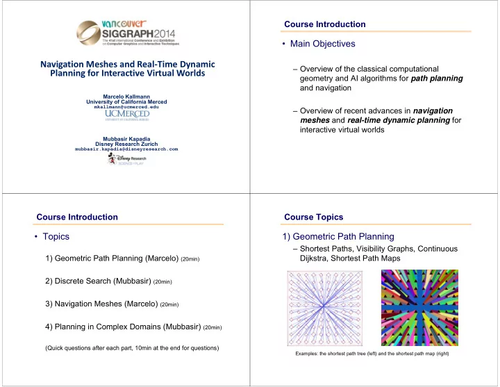
1) Geometric Path Planning

– Shortest Paths, Visibility Graphs, Continuous Dijkstra, Shortest Path Maps

Examples: the shortest path tree (left) and the shortest path map (right)

Course Topics

2) Discrete Search

– Extending classical A* to real-time constraints and dynamic scenarios, navigation with constraints, using GPU to speed up computations

Course Topics

3) Navigation Meshes

– Overview of approaches based on well established spatial structures

Example: Local Clearance Triangulations

Course Topics

4) Planning in Complex Domains

– Generalizing to complex navigation problems, and other problem domains, behavior planning, interactive narrative, etc.

Not in this Course

• Complementary Information

– More information on this course and related topics can be found from the webpages of the authors:

http://graphics.ucmerced.edu/ http://people.inf.ethz.ch/kapadiam/

– Course webpage:

http://people.inf.ethz.ch/kapadiam/2014-siggraph-course- navigation.html

• M. Kallmann

1

Geometric Path Planning

Marcelo Kallmann mkallmann@ucmerced.edu

http://graphics.ucmerced.edu/

• M. Kallmann

2

Geometric Path Planning

• Euclidean Shortest Paths (ESPs)

– Are collision-free shortest paths connecting two input points

• They are “globally” shortest, no shorter path will exist
• Navigation Meshes

– Several popular spatial structures can be used for fast path planning

• However usual structures will not compute ESPs
• Ex: Voronoi diagrams, medial axis, Delaunay

Triangulations

• M. Kallmann

3

Geometric Path Planning

Euclidean Shortest Paths (ESPs)

• M. Kallmann

Euclidean Shortest Paths

• Globally shortest paths are difficult to find

– The problem is a global continuous problem

• Cannot be efficiently reduced to graph search

– Most popular method

• Search the “Visibility Graph”, which unfortunately

has O(n2) size

– Can be solved in O(n log n)

• Using the “continuous Dijkstra” approach
• n = number of vertices in obstacle set
• Optimal algorithm difficult to implement in practice
• More about that later

4

• M. Kallmann

5

b

Euclidean Shortest Paths

a

• Simplest case: in a polygon
• M. Kallmann

6

b

Euclidean Shortest Paths

a

• Elastic band concept
• M. Kallmann

7

b

Euclidean Shortest Paths

a

• Elastic band concept
• M. Kallmann

8

b

Euclidean Shortest Paths

a

• Elastic band concept

• M. Kallmann

9

Euclidean Shortest Paths

b a

• Generic case: polygonal domain
• M. Kallmann

10

Euclidean Shortest Paths

a

• Multiple possible elastic bands exist

b

• M. Kallmann

11

Euclidean Shortest Paths

a

• Multiple possible elastic bands exist

b

• M. Kallmann

12

Euclidean Shortest Paths

a

• Multiple possible elastic bands exist

b

• M. Kallmann

13

Euclidean Shortest Paths

a

• Multiple possible elastic bands exist !!!

b

• M. Kallmann

14

Euclidean Shortest Paths

a

• How many?

b

• M. Kallmann

15

Euclidean Shortest Paths

a

• How many?

b

• M. Kallmann

16

Shortest Paths in a Simple Polygon

• M. Kallmann

17

Funnel Algorithm

• If we know the solution is in a given

polygon:

– Then there is a fast algorithm for finding the shortest path

• Funnel Algorithm

– Runs in optimal linear time

• M. Kallmann

18

Funnel Algorithm

x a

• M. Kallmann

19

Funnel Algorithm

• M. Kallmann

20

Funnel Algorithm

• M. Kallmann

21

Funnel Algorithm

• M. Kallmann

22

Funnel Algorithm

r b a

Deque: bar

• M. Kallmann

23

Funnel Algorithm

r b a

Deque: cbar

c

is (a,b,c) CCW?

• M. Kallmann

24

Funnel Algorithm

r b a

Deque: cbars

c

is (a,r,s) CW?

s

• M. Kallmann

25

Funnel Algorithm

r b a

Deque: dcbars

c s d

• M. Kallmann

26

Funnel Algorithm

r b a

Deque: dcbars

c s d e

(a,d,e) not CCW!

• M. Kallmann

27

Funnel Algorithm

r b a

Deque: ecbars

c s d e

• M. Kallmann

28

Funnel Algorithm

r b a

Deque: fbars

c s d e f

• M. Kallmann

29

Funnel Algorithm

r b a

Deque: fbars

c s d e f

• M. Kallmann

30

Funnel Algorithm

r b a

Deque: grs Path: a

c s d e f g

• M. Kallmann

31

Funnel Algorithm

r b a c s d e f g t

Deque: grst Path: a

• M. Kallmann

32

Funnel Algorithm

r b a c s d e f g t h

Deque: hst Path: ar

• M. Kallmann

33

Funnel Algorithm

r b a c s d e f g t h u

Deque: hu Path: ars

• M. Kallmann

34

Funnel Algorithm

r b a c s d e f g t h u i

Deque: ihu Path: ars

• M. Kallmann

35

Funnel Algorithm

r b a c s d e f g t h u i v

Deque: ihuv Path: ars

• M. Kallmann

36

Funnel Algorithm

r b a c s d e f g t h u i v j

Deque: juv Path: arsh

• M. Kallmann

37

Funnel Algorithm

r b a c s d e f g t h u i v j x

x reached!

Deque: jv Path: arshu

• M. Kallmann

38

Funnel Algorithm

r b a c s d e f g t h u i v j x

Path: arshux

• M. Kallmann

39

Funnel Algorithm

Result:

• M. Kallmann

40

Euclidean Shortest Paths

• Solving the generic ESP problem is more

difficult

– Popular algorithms in practice are based on the Visibility graph, which is O(n2) structure

• First build the visibility graph, then the shortest path

connecting two points in the graph will be the ESP

• M. Kallmann

41

Visibility Graph

• M. Kallmann

42

Visibility Graph

• Edges connect all pairs of visible vertices
• M. Kallmann

43

Visibility Graph

• M. Kallmann

44

Visibility Graph

• It can be preprocessed

– Query points added later at run-time

• M. Kallmann

45

Visibility Graph

• Full visibility graph

– Optimizations are possible

p q

• M. Kallmann

46

Visibility Graph

• Optimizations are possible

– Ex: discard edges connecting “concave corners”

p q

• M. Kallmann

47

Visibility Graph

• Final graph for path search

– Ready for a discrete path search algorithm

q p

• M. Kallmann

48

Visibility Graph

• Shortest Path in Graph

– Dijkstra and A* very popular

• Expansion outwards from source vertex
• Priority queue sorts nodes being expanded

1 2 4 6 8

1 1 2 2 2 1

3 5

2 2 3 3 3 3

7

• M. Kallmann

49

Visibility Graph

Q:

p q

1 2 4 6 8

1 1 2 2 2 1

3 5

2 2 3 3 3 3

7

• M. Kallmann

50

Visibility Graph

Q: 1

1 2 4 6 8 3 5 7

p

• M. Kallmann

51

Visibility Graph

Q:

1 2 4 6 8 3 5

s q

7

• M. Kallmann

52

Visibility Graph

Q:

1 2 4 6 8 3 5

s

7

• M. Kallmann

53

Visibility Graph

Q:

1 2 4 6 8 3 5

s

7

• M. Kallmann

54

Visibility Graph

Q: 4 2 3

1 2 4 6 8 3 5

s

7

g(n) is the cost-to-come h(n,q): cost-to-go heuristic, usually dist(n,q) (if zero: becomes Dijkstra algorithm)

• M. Kallmann

55

Visibility Graph

Q: 2 3

1 2 4 6 8 3 5

s

7

• M. Kallmann

56

Visibility Graph

Q: 2 3

1 2 4 6 8 3 5

s

7

• M. Kallmann

57

Visibility Graph

Q: 2 3 5 6

1 2 4 6 8 3 7 5

s

• M. Kallmann

58

Visibility Graph

Q: 3 5 6

1 2 4 6 8 3 7 5

s

node 2 has no neighbors to process

• M. Kallmann

59

Visibility Graph

Q: 5 6

1 2 4 6 8 3 7 5

s

• M. Kallmann

60

Visibility Graph

Q: 5 6 7

1 2 4 6 8 3 7 5

s

• M. Kallmann

61

Visibility Graph

Q: 6 7

1 2 4 6 8 3 7 5

s

• M. Kallmann

62

Visibility Graph

Q: 8 6 7

1 2 4 6 8 3 7 5

s

• M. Kallmann

63

Visibility Graph

Q: 6 7

1 2 4 6 8 3 7 5

s

• M. Kallmann

64

Visibility Graph

Q: 6 7

1 2 4 6 8 3 7 5

s q

When goal is reached, path is defined by tracing back parent pointers set during expansion

• M. Kallmann
• Search runs until goal node is reached

– In the worst case all nodes are visited

• Shortest path in Visibility Graph

– Is the ESP

Visibility Graph

65

• M. Kallmann
• Preprocessing for a specific clearance value

– Lozano-Pérez and Wesley 1979 – Chew 1985

• First dilates the environment, then computes visibility

graph of tangents

– Pre-computation: O(n2 log n), size: O(n2), query: O(n2 log n)

• Clearance-independent preprocessing possible

– Wein, van den Berg and Halperin, “the visibility– Voronoi complex and its applications”, 2007

• Preprocessing: O ( n2 log n )
• Query time: O ( n log n + m ) = O ( n2 )
• Probably the best practical method for global optimality

Visibility Graph

66

• M. Kallmann

67

Shortest Path Tree

• M. Kallmann

68

The Shortest Path Tree

• Contains shortest paths from all vertices to

source point

– Can be computed from the visibility graph with an exhaustive Dijkstra Expansion

• M. Kallmann

69

The Shortest Path Tree: Example

• M. Kallmann

70

The Shortest Path Tree

• The SPT is rooted at some source point
• Given a destination point,

how to use the SPT ?

– First compute visible vertices V to query point – Identify vertex vV that is in the shortest path to source point

• Simple given that vertices store their geodesic

distances to the SPT source (cost g)

– Shortest path is branch passing by v

• M. Kallmann

71

The Shortest Path Tree: Example

• M. Kallmann

72

Continuous Dijkstra

• M. Kallmann

73

Continuous Dijkstra

• Addresses the whole plane
• Principle is the same as discrete SPT

– But is continuous, will generate a Shortest Path Map (SPM) partition of the plane in O(n) cells

• Represents all shortest paths from the source to any

point in the continuous plane

• Once the SPM is computed, ESPs to the source

point can be efficiently computed

– It is based on the simulation of a “continuous wavefront propagation” from the source point

[Mitchell 1991; Mitchell 1993], [Hershberger and Suri 1997]

• M. Kallmann

74

Continuous Dijkstra

• Wavefront propagation

– Every point in the wavefront border has equal distance to the source point p

p

• M. Kallmann

75

Continuous Dijkstra

• Wavefront propagation

– Vertices hit by the wavefront will be visible to their wave generators

• M. Kallmann

76

Continuous Dijkstra

• Wavefront propagation

– Every time a vertex is reached, a new wave generator will cover the unseen region from the previous generator

• M. Kallmann

77

Continuous Dijkstra

• Wavefront propagation

– New vertices are processed as they are reached

• M. Kallmann

78

Continuous Dijkstra

• Wavefront propagation

– New vertices are processed as they are reached

• M. Kallmann

79

Continuous Dijkstra

• Wavefront propagation

– All points in the wavefront border remain with equal geodesic distance to the source point

• M. Kallmann

80

Continuous Dijkstra

• Front will eventually collide with itself

forming hyperbolic frontiers

Front collisions

• M. Kallmann

81

Continuous Dijkstra

• Result: Shortest Path Map

– Captures all possible shortest paths to the source point

• M. Kallmann

82

Continuous Dijkstra

• Path extraction from SPM

– First find region containing goal point, then trace back generator vertices

q

p

• M. Kallmann

83

Continuous Dijkstra: Example

• M. Kallmann

Continuous Dijkstra: Example

84

• M. Kallmann

Continuous Dijkstra: Example

85

q

p

• M. Kallmann

Continuous Dijkstra: Example

86 Camporesi and Kallmann, Computing Shortest Path Maps with GPU Shaders, under review.

• M. Kallmann

87

Geometric Path Planning

Summary

• M. Kallmann

88

Spatial Partitioning Structures

• Euclidean Shortest Paths are difficult to be

computed efficiently

– Simpler algorithms are related to the Visibility Graph, which is a O(n2) structure – Faster algorithms exist based on the Continuous Dijkstra approach, but they remain difficult to implement

• GPU-based examples showed

– As a result, most methods used in virtual environments do not attempt to compute ESPs

• Instead they focus on efficient path computation

• M. Kallmann

89

Questions?

• M. Kallmann

90

Thank You

• M. Kallmann

Navigation Meshes

Marcelo Kallmann mkallmann@ucmerced.edu

http://graphics.ucmerced.edu/

• M. Kallmann

Navigation Meshes

• Popular but not well defined

– Any “mesh” designed to support path and navigation queries can be referred to as a navigation mesh

• Since it is called a mesh, it is expected that some type
• f cell decomposition is used
• Alternatives

– Grids

• Simple and robust, but may be slow, too many cells

– Waypoints or roadmaps

• Fast, but they do not well represent spatial information

2

• M. Kallmann

Navigation Meshes

• Most solutions will be reduced to graph

search

– Roadmaps or waypoints directly define a graph to be searched – Navigation meshes will generate some sort of adjacency graph that is then used for path search – There are always difficulties to address

3

• M. Kallmann

Example

• Graph below well represents free space

– Such a graph could be extracted from a navigation mesh, from waypoints, etc.

4

• M. Kallmann

Example

• Given two query points

– Connect them to their closest points in the graph – Then run a graph search algorithm

5

• M. Kallmann

Example

• Shortest path in the graph

– Represents a valid collision-free path

6

• M. Kallmann

Example

• However the path is not the shortest one

– And it even misses the straight line solution !

7

• M. Kallmann

Example

• However the path is not the shortest one

– Path can be optimized to its locally optimal version, but it will still miss the global solution

8

• M. Kallmann

Navigation Meshes

• Navigation meshes in practice

– Properties are often difficult to define – Most methods have many special cases

• Difficult to account for all of them

– Computed paths often do not have clear properties besides being collision-free

• They are often only loosely defined to be “short”

9

• M. Kallmann

Next Topics

• Review of known structures suitable for fast

for path planning

– Medial Axis, Voronoi Diagram – Delaunay Triangulations

• Analysis of these structures when they are

used as navigation meshes

– Analysis of expected properties – Review of techniques and methods

10

• M. Kallmann

Medial Axis and CDTs

• M. Kallmann

Voronoi Diagram and Medial Axis

• Voronoi Diagram

– Given seed points, it will partition the plane in cells such that for each seed there will be a corresponding cell consisting of all points closer to that seed than to any other

• Generalized Voronoi diagram

– Generalization for edges as seeds

• Medial Axis

– The medial axis can be extracted from the Voronoi cell boundaries

12

• M. Kallmann

Voronoi Diagram and Medial Axis

– Medial axis can be extracted from the boundaries of the Voronoi diagram

Source of images: http://gamma.cs.unc.edu/VORONOI/ [Fast Computation of Generalized Voronoi Diagrams Using Graphics Hardware, Kenneth E. Hoff III, Tim Culver, John Keyser, Ming Lin, and Dinesh Manocha, SIGGRAPH’ 99] 13

Generalized Voronoi with a Maximal Clearance Path shown Voronoi of Seed Points

• M. Kallmann

Voronoi Diagram and Medial Axis

• Voronoi Diagram

– Several algorithms exist

• O(n) size, O(n log n) computation time

– Covered in several computational geometry textbooks

• Generalized Voronoi Diagram

– Methods using the graphics hardware often used

• Ex: Hoff et al. “Fast computation of generalized Voronoi

diagrams using graphics hardware”, 1999

– Medial axis can be easily extracted from the generalized Voronoi Diagram

14

• M. Kallmann

The Medial Axis

– Captures all paths of maximum clearance

(medial axis inside obstacles not shown)

15

• M. Kallmann

The Medial Axis

– Partition with segments to closest features

(medial axis inside obstacles not shown)

16

• M. Kallmann

The Delaunay Triangulation

• Delaunay Triangulations (DTs)

– DT will maximize the minimum internal angle of its triangles – DT is the dual of the Voronoi diagram

• Similar properties

– Extensive research on DTs available

• Constrained Delaunay Triangulations (CDTs)

– Allow to represent obstacle edges

17

• M. Kallmann

DT can be used to place and track moving agents for collision avoidance CDT can be used to represent the free environment, for navigation and path planning

Constrained Delaunay Triangulation

For every vertex, its closest vertex is connected by an edge CDT decomposes the free space in O(n) triangles

18

• M. Kallmann

DT can be used to place and track moving agents for collision avoidance CDT can be used to represent the free environment, for navigation and path planning

Circumcircles are all empty

Constrained Delaunay Triangulation

19

• M. Kallmann

DT can be used to place and track moving agents for collision avoidance CDT can be used to represent the free environment, for navigation and path planning

Vertices that are not visible to a triangle vertex may be inside a circumcircle Circumcircles are all empty

Constrained Delaunay Triangulation

20

• M. Kallmann

– Conformal decomposition of the free space – Number of triangles is O(n)

Constrained Delaunay Triangulation

21

• M. Kallmann

Navigation Meshes

• M. Kallmann

Navigation Meshes

• Navigation meshes are a representation of

the free environment

– For virtual worlds, being fast is most important

• Computing ESPs is usually not addressed
• What properties should we expect?

23

• M. Kallmann

Summary of Expected Properties

• Linear number of cells

– Critical for path search to run in optimal times

• Quality of paths

– Locally shortest paths should be provided

• Arbitrary clearance

– Same structure should handle any clearance value

• Representation robustness

– Intersections, overlaps, etc. should be handled

• Dynamic updates

– Efficient updates when environment changes

24

• M. Kallmann

Navigation Meshes

• Navigation meshes based on the Medial Axis

and on CDTs can provide such properties

25

• M. Kallmann

Navigation Meshes based on the Medial Axis

• M. Kallmann

Medial Axis

• Methods based on the medial axis

– Good choice when paths of maximum clearance are important – Paths with arbitrary clearance can be obtained – Medial axis is composed of straight line segments and parabolic arcs

27

• M. Kallmann

Medial Axis

• Methods based on the medial axis

– Graph search applied to the medial axis graph – Locally shortest solution can be then obtained

• For example by using Funnel algorithm

28

Maximum clearance path

• M. Kallmann

Medial Axis

• Methods based on the medial axis

– Graph search applied to the medial axis graph – Locally shortest solution can be then obtained

• For example by using Funnel algorithm

29

Locally shortest path Maximum clearance path A family of in-between solutions can be obtained by interpolation

• M. Kallmann

Medial Axis

• Medial Axis as a navigation mesh

– Good amount of work available

• For ex.: extensions for multi layered environments

and for handling dynamic updates available

– Geraerts, “Planning Short Paths with Clearance using Explicit Corridors”, 2010 – van Toll et al., “Navigation Meshes for Realistic Multi-Layered Environments”, 2011 – van Toll et al., “A Navigation Mesh for Dynamic Environments”, 2012

30

• M. Kallmann

Triangulations as Navigation Meshes

• M. Kallmann

Triangulations

• Triangulations as navigation meshes

– Triangle meshes are relatively simple to build

• Are composed of only straight edges

– Paths can be easily computed

• However handling clearance is not straightforward

– Can easily generate locally shortest paths

• For instance corridors will be already triangulated and

ready for the Funnel algorithm

– Extensive amount of work on the topic available

32

• M. Kallmann

Triangulations

• However, clearance not directly represented

– Edge lengths not enough

• Even if additional free edges are inserted to improve

capturing clearance in corridors

[Lamarche and Donikian, “Crowd of Virtual Humans: a New Approach for Real Time Navigation in Complex and Structured Environments”, 2004]

– Traversal clearance metrics possible

• Traversal clearance metric already used

[Demyen and Buro, “Efficient triangulation-based pathfinding”, 2006]

• However, as we are going to see, it does not work in

CDTs for all cases

• In addition, efficient clearance storage desirable

33

• M. Kallmann

Triangulations

• Local Clearance Triangulations (LCTs)

– Proposes a refinement strategy for CDTs allowing clearance information to be stored in the triangulation – Introduced in SCA 2010

• Kallmann, “Shortest Paths with Arbitrary Clearance

from Navigation Meshes”, 2010

– New results in TOG 2014

• Kallmann, “Dynamic and Robust Local Clearance

Triangulations”, 2014

– Being presented Wednesday 9AM session “Layout Building & Scenes”

34

• M. Kallmann

Local Clearance Triangulations

• Clearance Defined per triangle traversal

– Traversal from ab to bc: – Traversal clearance: s is the constraint behind ac and closest to b

35

• M. Kallmann

Local Clearance Triangulations

• However clearance metric not enough…

– Clearance in the red arrow direction not well captured

36

Traversal disturbance Triangle being traversed

• M. Kallmann

Local Clearance Triangulations

• But it can work if there are no disturbances

– By refining the triangulation disturbances can be eliminated and correct paths are obtained

37

• M. Kallmann

Local Clearance Triangulations

• Refinements solve disturbances

– Disturbances appear when a traversal does not correctly captures the local clearance of all possible exit directions

38

Traversal disturbance

• M. Kallmann

Local Clearance Triangulations

• Refinements solve disturbances

– Now all disturbances have been eliminated with refinements – Correct result: no valid path exists

39

New traversal now correctly captures narrow passage

• M. Kallmann

Local Clearance Triangulations

• Example of refinements

40

• M. Kallmann

LCT Channel Search

41

• M. Kallmann

Channel search: A* with “mid-edge metric” adjacency graph shown

LCT Channel Search

42

• M. Kallmann

Channel search: A* expansion

LCT Channel Search

43

• M. Kallmann

Channel search: each expansion performs the clearance test =>Clearance values stored in the triangulation, 2 scalars/edge

LCT Channel Search

44

• M. Kallmann

LCT Channel Search

45

Channel search: each expansion performs the clearance test

• M. Kallmann

LCT Channel Search

46

Channel search: expansions without enough clearance are not allowed

• M. Kallmann

LCT Channel Search

47

Channel search: expansions without enough clearance are not allowed

• M. Kallmann

LCT Channel Search

48

• M. Kallmann

LCT Channel Search

49

Channel search: done when goal point is reached

• M. Kallmann

LCT Channel Search

50

Channel search: result

• M. Kallmann

LCT Channel Search

51

Channel search: result

• M. Kallmann

Example LCT

52

• M. Kallmann

Example LCT

53

• M. Kallmann

Example LCT

54

• M. Kallmann

Example LCT

Test environment for The Sims 4: each small square represents a static character, later dynamically removed when it is time to walk

[used with permission] 55

• M. Kallmann

New Results on LCTs

Wednesday 9AM session “Layout Building & Scenes”

56

– Dynamic Operations with management of refinements – Robust operations addressing self-intersections at run-time – Optimizations and theoretical analysis

• M. Kallmann

Other Approaches for Navigation Meshes

• M. Kallmann

Additional Approaches

• Many other approaches are possible

– Ex.: coarser cell decompositions

• Lead to adjacency graphs with less nodes to search
• But becomes difficult to efficiently represent spatial

information such as arbitrary clearance

• Ex: NEOGEN approach

– Oliva and Pelechano, NEOGEN: Near Optimal Generator of Navigation Meshes for 3D Multi-Layered Environments, 2013 – Oliva and Pelechano, “A Generalized Exact Arbitrary Clearance Technique for Navigation Meshes”, 2013

58

• M. Kallmann

Additional Approaches

• Many other approaches are possible

– Impressive solutions for path planning have been developed

• Custom solutions for games, commercial packages

– But underlying techniques mostly remain similar to the standard ones

• Ex.: Recast & Detour toolkit

59

• M. Kallmann

Summary

• M. Kallmann

Summary

• Many approaches to efficient navigation

meshes are possible

– However it is difficult to achieve well-defined properties for the generated paths

• We covered a brief overview of methods

based on well-known spatial structures

– Medial axis offers paths of maximum clearance – LCTs can store clearance information in triangulations

61

• M. Kallmann

62

Questions?

• M. Kallmann

63

Thank You

Discrete Search for Interactive Game Applications

Mubbasir Kapadia

http://people.inf.ethz.ch/kapadiam/

http://people.inf.ethz.ch/kapadiam/2014-siggraph-course-navigation.html

Challenges

Real-time Planning in Dynamic Environments Planning with Constraints Scaling to large worlds and many agents

http://people.inf.ethz.ch/kapadiam/2014-siggraph-course-navigation.html

Real-time Planning in Dynamic Environments Planning with Constraints Scaling to large worlds and many agents

Proposed Solutions

From Classical A* to Anytime Dynamic Search

http://people.inf.ethz.ch/kapadiam/2014-siggraph-course-navigation.html

Real-time Planning in Dynamic Environments Planning with Constraints Scaling to large worlds and many agents

Proposed Solutions

From Classical A* to Anytime Dynamic Search Constraint-Aware Navigation in Dynamic Environments

http://people.inf.ethz.ch/kapadiam/2014-siggraph-course-navigation.html

Real-time Planning in Dynamic Environments Planning with Constraints Scaling to large worlds and many agents

Proposed Solutions

From Classical A* to Anytime Dynamic Search Constraint-Aware Navigation in Dynamic Environments Anytime Dynamic Search on the GPU

http://people.inf.ethz.ch/kapadiam/2014-siggraph-course-navigation.html

Real-time Planning in Dynamic Environments Planning with Constraints Scaling to large worlds and many agents

Proposed Solutions

From Classical A* to Anytime Dynamic Search Constraint-Aware Navigation in Dynamic Environments Anytime Dynamic Search on the GPU

http://people.inf.ethz.ch/kapadiam/2014-siggraph-course-navigation.html

From Classical A* to AD*

• A* with inflated heuristics
• Generalizing A* to include node inconsistency
• Anytime Search: provides sub-optimal solutions

while satisfying strict time constraints, with bounds on optimality.

• Dynamic Search: incrementally repairs solution to

accommodate dynamic environment changes

• Anytime Dynamic Search: combines anytime and

incremental properties

http://people.inf.ethz.ch/kapadiam/2014-siggraph-course-navigation.html

A* Search Algorithm

Computes optimal g-values of relevant states

http://people.inf.ethz.ch/kapadiam/2014-siggraph-course-navigation.html

Effect of Heuristic Function

• A* Search: expands states in order of f = g +h values
• Dijkstra’s: expands state in the order of f = g values
• Weighted A*: expands states in the order of f = g + ε.h values

– ε > 1 bias towards states that are closer to goal

http://people.inf.ethz.ch/kapadiam/2014-siggraph-course-navigation.html

Dijkstra’s Search Expansion

Expands state in the order of f = g values

Courtesy Likhachev 2010

http://people.inf.ethz.ch/kapadiam/2014-siggraph-course-navigation.html

A* Search Expansion

Expands state in the order of f = g+h values

Courtesy Likhachev 2010

http://people.inf.ethz.ch/kapadiam/2014-siggraph-course-navigation.html

A* Search Expansion

Expands state in the order of f = g+h values

Courtesy Likhachev 2010

For large problems, this results in A* quickly running out of memory

http://people.inf.ethz.ch/kapadiam/2014-siggraph-course-navigation.html

Weighted A* Search Expansion

Expands states in the order of f = g + ε.h values ε > 1 bias towards states that are closer to goal

Courtesy Likhachev 2010

http://people.inf.ethz.ch/kapadiam/2014-siggraph-course-navigation.html

Anytime Repairing A* (ARA*)

Efficient series of weighted A* searches with decreasing ε

http://people.inf.ethz.ch/kapadiam/2014-siggraph-course-navigation.html

Anytime Repairing A* (ARA*)

Efficient series of weighted A* searches with decreasing ε

ARA*: Anytime A* with Provable Bounds on Sub-Optimality Maxim Likhachev, Geoff Gordon and Sebastian Thrun Advances in Neural Information Processing Systems, 2003 http://people.inf.ethz.ch/kapadiam/2014-siggraph-course-navigation.html

Anytime Repairing A* (ARA*)

http://people.inf.ethz.ch/kapadiam/2014-siggraph-course-navigation.html

Anytime Repairing A* (ARA*)

Consistent State: Inconsistent State:

http://people.inf.ethz.ch/kapadiam/2014-siggraph-course-navigation.html

Anytime Repairing A* (ARA*)

http://people.inf.ethz.ch/kapadiam/2014-siggraph-course-navigation.html

Anytime Repairing A* (ARA*)

http://people.inf.ethz.ch/kapadiam/2014-siggraph-course-navigation.html

Anytime D*

Set ε to large value While goal is not reached ComputePathWithReuse() Publish ε-suboptimal path Follow path until map is updated Update corresponding edge costs Set start to current state of agent If significant changes were observed Increase ε or replan from scratch Else Decrease ε Combined properties of anytime and dynamic planning

Anytime search in dynamic graphs Maxim Likhachev, Dave Ferguson, Geoff Gordon, Anthony Stentz, and Sebastian Thrun Journal of Artificial Intelligence, 2008

http://people.inf.ethz.ch/kapadiam/2014-siggraph-course-navigation.html

Anytime D*

Set ε to large value While goal is not reached ComputePathWithReuse() Publish ε-suboptimal path Follow path until map is updated Update corresponding edge costs Set start to current state of agent If significant changes were observed Increase ε or replan from scratch Else Decrease ε Combined properties of anytime and dynamic planning

Anytime search in dynamic graphs Maxim Likhachev, Dave Ferguson, Geoff Gordon, Anthony Stentz, and Sebastian Thrun Journal of Artificial Intelligence, 2008 http://people.inf.ethz.ch/kapadiam/2014-siggraph-course-navigation.html

Anytime D*

Set ε to large value While goal is not reached ComputePathWithReuse() Publish ε-suboptimal path Follow path until map is updated Update corresponding edge costs Set start to current state of agent If significant changes were observed Increase ε or replan from scratch Else Decrease ε Combined properties of anytime and dynamic planning

Anytime search in dynamic graphs Maxim Likhachev, Dave Ferguson, Geoff Gordon, Anthony Stentz, and Sebastian Thrun Journal of Artificial Intelligence, 2008 http://people.inf.ethz.ch/kapadiam/2014-siggraph-course-navigation.html

Anytime D*

Set ε to large value While goal is not reached ComputePathWithReuse() Publish ε-suboptimal path Follow path until map is updated Update corresponding edge costs Set start to current state of agent If significant changes were observed Increase ε or replan from scratch Else Decrease ε Combined properties of anytime and dynamic planning

Anytime search in dynamic graphs Maxim Likhachev, Dave Ferguson, Geoff Gordon, Anthony Stentz, and Sebastian Thrun Journal of Artificial Intelligence, 2008 http://people.inf.ethz.ch/kapadiam/2014-siggraph-course-navigation.html

Anytime D*

http://people.inf.ethz.ch/kapadiam/2014-siggraph-course-navigation.html

Inflated Heuristics

http://people.inf.ethz.ch/kapadiam/2014-siggraph-course-navigation.html

Node Inconsistency

http://people.inf.ethz.ch/kapadiam/2014-siggraph-course-navigation.html

Anytime Search: ARA*

http://people.inf.ethz.ch/kapadiam/2014-siggraph-course-navigation.html

Anytime Search: ARA*

http://people.inf.ethz.ch/kapadiam/2014-siggraph-course-navigation.html

Anytime Search: ARA*

http://people.inf.ethz.ch/kapadiam/2014-siggraph-course-navigation.html http://people.inf.ethz.ch/kapadiam/2014-siggraph-course-navigation.html

Anytime Dynamic Search: AD*

http://people.inf.ethz.ch/kapadiam/2014-siggraph-course-navigation.html

Real-time Planning in Dynamic Environments Planning with Constraints Scaling to large worlds and many agents

Proposed Solutions

From Classical A* to Anytime Dynamic Search Constraint-Aware Navigation in Dynamic Environments Anytime Dynamic Search on the GPU

http://people.inf.ethz.ch/kapadiam/2014-siggraph-course-navigation.html

Global Navigation with Spatial Constraints in Dynamic Environments

http://people.inf.ethz.ch/kapadiam/2014-siggraph-course-navigation.html

Extending AD* to compute and repair constraint-aware paths

http://people.inf.ethz.ch/kapadiam/2014-siggraph-course-navigation.html

Challenges

Environment representation Constraint specification Constraint Satisfaction

http://people.inf.ethz.ch/kapadiam/2014-siggraph-course-navigation.html

Prior Work

• Potential Fields [Warren 1989, Warren 1990, Shimoda et
• al. 2005, Goldenstein et al. 2001, Arkin 1987]

– Dynamic Potential Fields [Treuille et al. 2006] – Local variable-resolution fields [Kapadia et al. 2009,

2012]

http://people.inf.ethz.ch/kapadiam/2014-siggraph-course-navigation.html

Prior Work

• Discrete Search Methods [Hart et al. 1968, 1972,

Dechter and Pearl 1985]

– Reduced branching factor [Lau and Kuffner 2005; Lo

and Zwicker 2008, Kapadia et al. 2013]

– Triangulations [Mononen 2009; Kallmann 2010, Olivana

and Pelechano 2013]

– Anytime Planning [Likhachev et al. 2003; van den Berg

et al. 2006, Safonova and Hodgins 2007]

– Incremental Planning [Koenig and Likhachev 2002]

http://people.inf.ethz.ch/kapadiam/2014-siggraph-course-navigation.html

Prior Work

• Hierarchical Planning [Botea et al. 2004;Bulitko et al.

2007; Holte et al. 1996]

– Heuristic computation in high-level graphs [Holte et

• al. 1996]

– Waypoints as intermediate goals [Singh et al. 2011;

Choi et al. 2011]

– Tunnel search [Gochev et al. 2011]

http://people.inf.ethz.ch/kapadiam/2014-siggraph-course-navigation.html

Prior Work

• Local Collision Avoidance [Pelechano et al. 2008;

Thalmann 2008]

– Reactive approaches [Reynolds 1987; Lamarche and

Donikian 2004; Loscos et al. 2003]

– Social forces [Helbing and Molnar 1995; Pelechano et al.

2007]

– Predictive approaches [van den Berg et al. 2008; Paris et

• al. 2007, Singh et al. 2011]

http://people.inf.ethz.ch/kapadiam/2014-siggraph-course-navigation.html

Prior Work

• Navigation with Constraints [Al Marzouqi and Jarvis

2011]

– Spatial semantics [Andre et al. 1986, Xu and Badler 2000] – Homotopy based search [Bhattacharya et al. 2012a,

2012b]

– HA* [Hernandez et al. 2011] – Experience Graphs [Phillips et al. 2013] – Clearance constraints [Geraerts 2010; Kallmann 2010,

Oliva and Pelechano 2013]

http://people.inf.ethz.ch/kapadiam/2014-siggraph-course-navigation.html

Proposed Solutions

Environment representation Constraint specification Constraint Satisfaction Hybrid representation for constraint- aware navigation

http://people.inf.ethz.ch/kapadiam/2014-siggraph-course-navigation.html

Proposed Solutions

Environment representation Constraint specification Constraint Satisfaction Hybrid representation for constraint- aware navigation Cost multiplier fields used to represent qualitative constraints

http://people.inf.ethz.ch/kapadiam/2014-siggraph-course-navigation.html

Proposed Solutions

Environment representation Constraint specification Constraint Satisfaction Hybrid representation for constraint- aware navigation Cost multiplier fields used to represent qualitative constraints An anytime dynamic planner that computes and repairs constraint-aware paths

http://people.inf.ethz.ch/kapadiam/2014-siggraph-course-navigation.html

Problem Definition

Problem Domain: Problem Definition: Planning Task: Compute from that satisfies

http://people.inf.ethz.ch/kapadiam/2014-siggraph-course-navigation.html

Problem Definition

Problem Domain: Problem Definition: Planning Task: Compute from that satisfies

http://people.inf.ethz.ch/kapadiam/2014-siggraph-course-navigation.html

Annotated Environment

http://people.inf.ethz.ch/kapadiam/2014-siggraph-course-navigation.html

Wavefront expansion. N =3 Hybrid Environment Discretization

http://people.inf.ethz.ch/kapadiam/2014-siggraph-course-navigation.html

Problem Definition

Problem Domain: Problem Definition: Planning Task: Compute from that satisfies

http://people.inf.ethz.ch/kapadiam/2014-siggraph-course-navigation.html

Wavefront expansion. N =3 Problem Definition with Constraints

http://people.inf.ethz.ch/kapadiam/2014-siggraph-course-navigation.html

Problem Definition

Problem Domain: Problem Definition: Planning Task: Compute from that satisfies

http://people.inf.ethz.ch/kapadiam/2014-siggraph-course-navigation.html

Plan without constraint satisfaction

http://people.inf.ethz.ch/kapadiam/2014-siggraph-course-navigation.html

Plan with constraint satisficaction

http://people.inf.ethz.ch/kapadiam/2014-siggraph-course-navigation.html

Wavefront expansion. N =3

http://people.inf.ethz.ch/kapadiam/2014-siggraph-course-navigation.html

Wavefront expansion. N =3

http://people.inf.ethz.ch/kapadiam/2014-siggraph-course-navigation.html

Wavefront expansion. N =3

Multiple paths with constraint variations

http://people.inf.ethz.ch/kapadiam/2014-siggraph-course-navigation.html

Environment Triangulation

http://people.inf.ethz.ch/kapadiam/2014-siggraph-course-navigation.html

Object annotations with additional nodes added to

http://people.inf.ethz.ch/kapadiam/2014-siggraph-course-navigation.html

Dense Uniform Graph

http://people.inf.ethz.ch/kapadiam/2014-siggraph-course-navigation.html

Hybrid graph

http://people.inf.ethz.ch/kapadiam/2014-siggraph-course-navigation.html

Constraint Properties

Modified cost of a transition must never be negative, to ensure that the search will complete. We must be able to efficiently compute the cost of a transition, influenced by several constraints. Constraints should only affect region of influence The total cost along a path must be independent of the number of states along that path

http://people.inf.ethz.ch/kapadiam/2014-siggraph-course-navigation.html

Constraint Properties

Modified cost of a transition must never be negative, to ensure that the search will complete. We must be able to efficiently compute the cost of a transition, influenced by several constraints. Constraints should only affect region of influence The total cost along a path must be independent of the number of states along that path

http://people.inf.ethz.ch/kapadiam/2014-siggraph-course-navigation.html

Constraint Properties

Modified cost of a transition must never be negative, to ensure that the search will complete. We must be able to efficiently compute the cost of a transition, influenced by several constraints. Constraints should only affect region of influence The total cost along a path must be independent of the number of states along that path Transition cost always greater than or equal to its un- modified distance cost

http://people.inf.ethz.ch/kapadiam/2014-siggraph-course-navigation.html

Constraint Properties

Modified cost of a transition must never be negative, to ensure that the search will complete. We must be able to efficiently compute the cost of a transition, influenced by several constraints. Constraints should only affect region of influence The total cost along a path must be independent of the number of states along that path Transition cost always greater than or equal to its un- modified distance cost

http://people.inf.ethz.ch/kapadiam/2014-siggraph-course-navigation.html

Constraint Properties

Modified cost of a transition must never be negative, to ensure that the search will complete. We must be able to efficiently compute the cost of a transition, influenced by several constraints. Constraints should only affect a limited region of influence The total cost along a path must be independent of the number of states along that path Weighted influence of all active constraints simply added together, and multiplied to base cost Transition cost always greater than or equal to its un- modified distance cost

http://people.inf.ethz.ch/kapadiam/2014-siggraph-course-navigation.html

Constraint Properties

Weighted influence of all active constraints simply added together, and multiplied to base cost Transition cost always greater than or equal to its un- modified distance cost Modified cost of a transition must never be negative, to ensure that the search will complete. We must be able to efficiently compute the cost of a transition, influenced by several constraints. Constraints should only affect a limited region of influence The total cost along a path must be independent of the number of states along that path

http://people.inf.ethz.ch/kapadiam/2014-siggraph-course-navigation.html

Constraint Properties

Weighted influence of all active constraints simply added together, and multiplied to base cost Transition cost always greater than or equal to its un- modified distance cost Constraints modeled as potential fields with gradient Modified cost of a transition must never be negative, to ensure that the search will complete. We must be able to efficiently compute the cost of a transition, influenced by several constraints. Constraints should only affect a limited region of influence The total cost along a path must be independent of the number of states along that path

http://people.inf.ethz.ch/kapadiam/2014-siggraph-course-navigation.html

Constraint Properties

Weighted influence of all active constraints simply added together, and multiplied to base cost Transition cost always greater than or equal to its un- modified distance cost Constraints modeled as potential fields with gradient Modified cost of a transition must never be negative, to ensure that the search will complete. We must be able to efficiently compute the cost of a transition, influenced by several constraints. Constraints should only affect a limited region of influence The total cost along a path must be independent of the number of states along that path

http://people.inf.ethz.ch/kapadiam/2014-siggraph-course-navigation.html

Constraint Formulation

http://people.inf.ethz.ch/kapadiam/2014-siggraph-course-navigation.html

Constraint Formulation

http://people.inf.ethz.ch/kapadiam/2014-siggraph-course-navigation.html

Constraint Formulation

http://people.inf.ethz.ch/kapadiam/2014-siggraph-course-navigation.html

Constraint Formulation

http://people.inf.ethz.ch/kapadiam/2014-siggraph-course-navigation.html

Constraint Formulation

http://people.inf.ethz.ch/kapadiam/2014-siggraph-course-navigation.html

Multiple Constraints

Cost multiplier for a transition:

http://people.inf.ethz.ch/kapadiam/2014-siggraph-course-navigation.html

Multiple Constraints

Cost multiplier for a transition:

http://people.inf.ethz.ch/kapadiam/2014-siggraph-course-navigation.html

Multiple Constraints

Cost multiplier for a transition:

http://people.inf.ethz.ch/kapadiam/2014-siggraph-course-navigation.html

Multiple Constraints

Cost multiplier for a transition:

http://people.inf.ethz.ch/kapadiam/2014-siggraph-course-navigation.html

Multiple Constraints

Cost multiplier for a transition:

http://people.inf.ethz.ch/kapadiam/2014-siggraph-course-navigation.html

Planner: Cost Computation

Modified cost of reaching state s:

http://people.inf.ethz.ch/kapadiam/2014-siggraph-course-navigation.html

Accommodating Dynamic Constraints

http://people.inf.ethz.ch/kapadiam/2014-siggraph-course-navigation.html

http://people.inf.ethz.ch/kapadiam/2014-siggraph-course-navigation.html http://people.inf.ethz.ch/kapadiam/2014-siggraph-course-navigation.html

Benefit of Hybrid Domain

http://people.inf.ethz.ch/kapadiam/2014-siggraph-course-navigation.html

Conclusion & Future Work

• A goal-directed navigation system that satisfies

multiple spatial constraints

• Computational performance sensitive to

triangulations and dense representation

• A hybrid approach to satisfying constraints for

global navigation and local collision avoidance

• Social Navigation for Autonomous Agents

http://people.inf.ethz.ch/kapadiam/2014-siggraph-course-navigation.html

Real-time Planning in Dynamic Environments Planning with Constraints Scaling to large worlds and many agents

Proposed Solutions

From Classical A* to Anytime Dynamic Search Constraint-Aware Navigation in Dynamic Environments Anytime Dynamic Search on the GPU

http://people.inf.ethz.ch/kapadiam/2014-siggraph-course-navigation.html

Need for high fidelity navigation in complex, dynamic virtual environments

http://people.inf.ethz.ch/kapadiam/2014-siggraph-course-navigation.html

Need for high fidelity navigation in complex, dynamic virtual environments A massively parallelizable planning framework with strict optimality guarantees and efficient plan repair

http://people.inf.ethz.ch/kapadiam/2014-siggraph-course-navigation.html

Challenges

Large-scale, complex, dynamic environments Strict optimality requirements Scalability with number of agents

http://people.inf.ethz.ch/kapadiam/2014-siggraph-course-navigation.html

Proposed Solutions

Large-scale, complex, dynamic environments Strict optimality requirements Scalability with number of agents

Massively parallel wave-front based search with efficient plan repair

http://people.inf.ethz.ch/kapadiam/2014-siggraph-course-navigation.html

Proposed Solutions

Large-scale, complex, dynamic environments Strict optimality requirements Scalability with number of agents

Massively parallel wave-front based search with efficient plan repair Termination condition enforces strict optimality with minimum number of GPU iterations

http://people.inf.ethz.ch/kapadiam/2014-siggraph-course-navigation.html

Proposed Solutions

Large-scale, complex, dynamic environments Strict optimality requirements Scalability with number of agents

Massively parallel wave-front based search with efficient plan repair Termination condition enforces strict optimality with minimum number of GPU iterations Handles any number of moving agents at no additional computational cost

http://people.inf.ethz.ch/kapadiam/2014-siggraph-course-navigation.html

Method Overview

http://people.inf.ethz.ch/kapadiam/2014-siggraph-course-navigation.html

Method Overview

http://people.inf.ethz.ch/kapadiam/2014-siggraph-course-navigation.html

Method Overview

http://people.inf.ethz.ch/kapadiam/2014-siggraph-course-navigation.html

Method Overview

http://people.inf.ethz.ch/kapadiam/2014-siggraph-course-navigation.html

Method Overview

http://people.inf.ethz.ch/kapadiam/2014-siggraph-course-navigation.html

Method Overview

http://people.inf.ethz.ch/kapadiam/2014-siggraph-course-navigation.html

Method Overview

http://people.inf.ethz.ch/kapadiam/2014-siggraph-course-navigation.html

Method Overview

http://people.inf.ethz.ch/kapadiam/2014-siggraph-course-navigation.html

Wavefront expansion. N =3

http://people.inf.ethz.ch/kapadiam/2014-siggraph-course-navigation.html

Wavefront expansion. N =11

http://people.inf.ethz.ch/kapadiam/2014-siggraph-course-navigation.html

Wavefront expansion. N =15

http://people.inf.ethz.ch/kapadiam/2014-siggraph-course-navigation.html

Wavefront expansion. N =18

http://people.inf.ethz.ch/kapadiam/2014-siggraph-course-navigation.html

Termination Conditions

Exit when goal reached Exit when whole map converges Minimal map convergence with optimality guarantees

http://people.inf.ethz.ch/kapadiam/2014-siggraph-course-navigation.html

Non-uniform state space

http://people.inf.ethz.ch/kapadiam/2014-siggraph-course-navigation.html

Sub-optimal solution, N = 8

http://people.inf.ethz.ch/kapadiam/2014-siggraph-course-navigation.html

Termination Conditions

Exit when goal reached Exit when whole map converges Minimal map convergence with optimality guarantees

http://people.inf.ethz.ch/kapadiam/2014-siggraph-course-navigation.html

Optimal solution, N = 17

http://people.inf.ethz.ch/kapadiam/2014-siggraph-course-navigation.html

Termination Conditions

Exit when goal reached Exit when whole map converges Minimal map convergence with optimality guarantees

http://people.inf.ethz.ch/kapadiam/2014-siggraph-course-navigation.html

Optimal solution, N = 12 (minimum number of iterations)

http://people.inf.ethz.ch/kapadiam/2014-siggraph-course-navigation.html

Efficient Plan Repair for Dynamic Environments & Moving Agents

http://people.inf.ethz.ch/kapadiam/2014-siggraph-course-navigation.html http://people.inf.ethz.ch/kapadiam/2014-siggraph-course-navigation.html

Multi-Agent Planning

Extended Termination Condition Multi-Agent Simulation

• Single map can be queried by all agents to compute path
• Movement along path using local collision avoidance

Multiple Target Locations

• A separate map required for each target
• Significant memory overhead

http://people.inf.ethz.ch/kapadiam/2014-siggraph-course-navigation.html

Performance Analysis

Agent Scalability Environment Scalability Memory Dynamic Planning

http://people.inf.ethz.ch/kapadiam/2014-siggraph-course-navigation.html

Scalability with Number of Agents

http://people.inf.ethz.ch/kapadiam/2014-siggraph-course-navigation.html

Scalability with Environment Size

http://people.inf.ethz.ch/kapadiam/2014-siggraph-course-navigation.html

Scalability with Environment Size

http://people.inf.ethz.ch/kapadiam/2014-siggraph-course-navigation.html

GPU Memory Requirement

http://people.inf.ethz.ch/kapadiam/2014-siggraph-course-navigation.html

Dynamic Planning

http://people.inf.ethz.ch/kapadiam/2014-siggraph-course-navigation.html http://people.inf.ethz.ch/kapadiam/2014-siggraph-course-navigation.html

http://people.inf.ethz.ch/kapadiam/2014-siggraph-course-navigation.html http://people.inf.ethz.ch/kapadiam/2014-siggraph-course-navigation.html

Conclusion

• A massively parallel wave-front based

planning technique which can efficiently handle world changes and agent movement by reusing previous computations

• Computational cost independent of number of

agents

• Memory overhead for multiple goals

http://people.inf.ethz.ch/kapadiam/2014-siggraph-course-navigation.html

GPU-based Dynamic Search on Adaptive Resolution Grids

GPU-based Dynamic Search on Adaptive Resolution Grids Francisco Garcia, Mubbasir Kapadia, and Norman I. Badler IEEE International Conference on Robotics and Automation, June 2014

Planning in Complex Domains

Mubbasir Kapadia

http://people.inf.ethz.ch/kapadiam/

http://people.inf.ethz.ch/kapadiam/2014-siggraph-course-navigation.html

• Footstep Domain for Dynamic Crowds
• Use of Multiple Control Domains for Higher

Control Fidelity

• Additional Examples

Outline

http://people.inf.ethz.ch/kapadiam/2014-siggraph-course-navigation.html

Footstep Domain for Dynamic Crowds Use of Multiple Control Domains for Higher Control Fidelity Additional Examples

Outline

http://people.inf.ethz.ch/kapadiam/2014-siggraph-course-navigation.html

“Current steering algorithms cannot handle the space of all possible scenarios that agents encounter in dynamic virtual environments”

Scenario Space: Characterizing Coverage, Quality, and Failure of Steering Algorithms Mubbasir Kapadia, Matt Wang, Shawn Singh, Glenn Reinmann, Petros Faloutsos ACM SIGGRAPH Symposium on Computer Animation, August 2011

http://people.inf.ethz.ch/kapadiam/2014-siggraph-course-navigation.html

“A particle-based agent representation cannot capture nuanced interactions that humans exhibit in confined and crowded situations.”

http://people.inf.ethz.ch/kapadiam/2014-siggraph-course-navigation.html

“A particle-based agent representation cannot capture nuanced interactions that humans exhibit in confined and crowded situations.”

http://people.inf.ethz.ch/kapadiam/2014-siggraph-course-navigation.html

“A particle-based agent representation cannot capture nuanced interactions that humans exhibit in confined and crowded situations.”

http://people.inf.ethz.ch/kapadiam/2014-siggraph-course-navigation.html

http://people.inf.ethz.ch/kapadiam/2014-siggraph-course-navigation.html

Footstep Navigation for Dynamic Crowds

Footstep Navigation for Dynamic Crowds Shawn Singh, Mubbasir Kapadia, Glenn Reinmann, Petros Faloutsos Special Issue, Computer Animation and Virtual Worlds (CAVW), April 2011 http://people.inf.ethz.ch/kapadiam/2014-siggraph-course-navigation.html

Footstep Domain

State and Action Space

http://people.inf.ethz.ch/kapadiam/2014-siggraph-course-navigation.html

Footstep Action Selection

http://people.inf.ethz.ch/kapadiam/2014-siggraph-course-navigation.html

Footstep Action Selection

http://people.inf.ethz.ch/kapadiam/2014-siggraph-course-navigation.html

Footstep Orientation

http://people.inf.ethz.ch/kapadiam/2014-siggraph-course-navigation.html

Cost Formulation

Cost Function Heuristic Function

http://people.inf.ethz.ch/kapadiam/2014-siggraph-course-navigation.html

Cost Formulation

Cost Function Heuristic Function

http://people.inf.ethz.ch/kapadiam/2014-siggraph-course-navigation.html

Spherical Inverted Pendulum Model – Sagittal View

http://people.inf.ethz.ch/kapadiam/2014-siggraph-course-navigation.html

Cost Formulation

Cost Function Heuristic Function

http://people.inf.ethz.ch/kapadiam/2014-siggraph-course-navigation.html

Cost Formulation

Cost Function Heuristic Function

http://people.inf.ethz.ch/kapadiam/2014-siggraph-course-navigation.html

Short Horizon Space-Time Planner

http://people.inf.ethz.ch/kapadiam/2014-siggraph-course-navigation.html

U Turn

http://people.inf.ethz.ch/kapadiam/2014-siggraph-course-navigation.html

Dynamic Collision Bounds

http://people.inf.ethz.ch/kapadiam/2014-siggraph-course-navigation.html

Narrow Passageways

http://people.inf.ethz.ch/kapadiam/2014-siggraph-course-navigation.html

Large Scale Simulations

http://people.inf.ethz.ch/kapadiam/2014-siggraph-course-navigation.html

Coverage Comparison

Scenario Space: Characterizing Coverage, Quality, and Failure of Steering Algorithms Mubbasir Kapadia, Matt Wang, Shawn Singh, Glenn Reinmann, Petros Faloutsos ACM SIGGRAPH Symposium on Computer Animation, August 2011

http://people.inf.ethz.ch/kapadiam/2014-siggraph-course-navigation.html

Need for high fidelity navigation in complex, dynamic virtual environments

http://people.inf.ethz.ch/kapadiam/2014-siggraph-course-navigation.html

The Quest for Complete Coverage

Scenario Space: Characterizing Coverage, Quality, and Failure of Steering Algorithms Mubbasir Kapadia, Matt Wang, Shawn Singh, Glenn Reinmann, Petros Faloutsos ACM SIGGRAPH Symposium on Computer Animation, August 2011 http://people.inf.ethz.ch/kapadiam/2014-siggraph-course-navigation.html

Footstep Domain for Dynamic Crowds Use of Multiple Control Domains for Higher Control Fidelity Additional Examples

Outline

http://people.inf.ethz.ch/kapadiam/2014-siggraph-course-navigation.html

Need for high fidelity navigation in complex, dynamic virtual environments Real-time system that can handle many characters, without compromising control fidelity.

http://people.inf.ethz.ch/kapadiam/2014-siggraph-course-navigation.html

Challenges

Problem domain of interacting autonomous agents is high-dimensional and continuous Tradeoff between action fidelity and scalability

Prior Work

• Global Navigation [Sung et al. 2005; Sud et al. 2007;

van den Berg et al. 2008b; Kallmann 2010]

– Efficient navigation in static environments

• Crowd Simulation [Pelechano et al. 2008; Thalmann

2008]

– Reactive approaches [Reynolds 1987; Lamarche and

Donikian 2004; Loscos et al. 2003]

– Predictive approaches [van den Berg et al. 2008; Paris

et al. 2007]

Prior Work

• Planning solutions [Choi et al. 2003;Fraichard 1999; Shapiro

et al. 2007]

– Few agents with complex action spaces

• Search acceleration

– Reduced branching factor [Lau and Kuffner 2005; Lo and

Zwicker 2008]

– Reduced search horizon [Singh et al. 2011; Choi et al. 2011] – Anytime Planning [Likhachev et al. 2003; van den Berg et al.

2006, Safonova and Hodgins 2007]

– Randomized Planners [Hsu et al. 2000; Shapiro et al. 2007]

Prior Work

• Hierarchical Planning [Botea et al. 2004;Bulitko et al.

2007; Holte et al. 1996]

– Heuristic computation in high-level graphs [Holte et

• al. 1996]

– Waypoints as intermediate goals [Singh et al. 2011;

Choi et al. 2011]

– Tunnel search [Gochev et al. 2011]

http://people.inf.ethz.ch/kapadiam/2014-siggraph-course-navigation.html

Proposed Solution

Multiple heterogeneous problem domains Problem domain of interacting autonomous agents is high-dimensional and continuous Tradeoff between action fidelity and scalability

Multi-Domain Real-Time Planning in Dynamic Environments Mubbasir Kapadia, Alejandro Porres, Francisco Garcia, Nuria Pelechano, Norman I. Badler ACM SIGGRAPH/EUROGRAPHICS Symposium of Computer Animation (SCA), 2013 http://people.inf.ethz.ch/kapadiam/2014-siggraph-course-navigation.html

Proposed Solution

Problem domain of interacting autonomous agents is high-dimensional and continuous Tradeoff between action fidelity and scalability Multi-Domain Anytime Dynamic Planning Framework Multiple heterogeneous problem domains

Multi-Domain Real-Time Planning in Dynamic Environments Mubbasir Kapadia, Alejandro Porres, Francisco Garcia, Nuria Pelechano, Norman I. Badler ACM SIGGRAPH/EUROGRAPHICS Symposium of Computer Animation (SCA), 2013

Problem Domain

State Space: Action Space: Cost: Heuristic:

Problem Instance

http://people.inf.ethz.ch/kapadiam/2014-siggraph-course-navigation.html

Problem Definition Σ1 : Static Navigation Mesh Domain Global Path Computation in Σ1 Σ2 : Dynamic Navigation Mesh Domain

Σ3 : Uniform Grid Domain Σ4 : Space-Time Domain Space-Time Domain

s = < x, v, t > s' = Δ ɵ t t+Δ t

v

< x+(v+Δ v).Δ t, v+Δ v, t+Δ t >

http://people.inf.ethz.ch/kapadiam/2014-siggraph-course-navigation.html

Domain Mapping

: polygon -> polygon(s) mapping : maps a polygon to multiple grid cells

http://people.inf.ethz.ch/kapadiam/2014-siggraph-course-navigation.html

Domain Mapping

: polygon -> polygon(s) mapping : maps a polygon to multiple grid cells

http://people.inf.ethz.ch/kapadiam/2014-siggraph-course-navigation.html

Domain Mapping

: polygon -> polygon(s) mapping : maps a polygon to multiple grid cells

http://people.inf.ethz.ch/kapadiam/2014-siggraph-course-navigation.html

Domain Mapping

: polygon -> polygon(s) mapping : maps a polygon to multiple grid cells

http://people.inf.ethz.ch/kapadiam/2014-siggraph-course-navigation.html

Mapping successive waypoints to independent planning tasks

http://people.inf.ethz.ch/kapadiam/2014-siggraph-course-navigation.html

Tunnels

Exploit low-dimensional plan to accelerate searches in high dimensional space by focusing in the neighborhood of the low dimensional plan

Planning subspace: Heuristic:

Path Planning with Adaptive Dimensionality Kalin Gochev, Benjamin Cohen, Jonathan Butzke, Alla Safanova, Maxim Likhachev AAAI Publications, Fourth Annual Symposium on Combinatorial Search

Problem Decomposition

T(∑

1)

T(∑

2)

T(∑

3)

T(∑

4)

TUNNEL CHANGE TUNNEL CHANGE TUNNEL CHANGE T(∑

1)

T(∑

2)

T(∑

3)

T(∑

4)

TUNNEL CHANGE START & GOAL CHANGES TUNNEL CHANGE T(∑

3)

T(∑

4)

TUNNEL CHANGE . . . . . .

Problem Decomposition Planning Task

LIKHACHEV, M., FERGUSON, D. I., GORDON, G. J., STENTZ, A., AND THRUN, S. 2005. Anytime Dynamic A*: An Anytime, Replanning Algorithm. ICAPS.

http://people.inf.ethz.ch/kapadiam/2014-siggraph-course-navigation.html

Task Priorities

http://people.inf.ethz.ch/kapadiam/2014-siggraph-course-navigation.html

Task Priorities

http://people.inf.ethz.ch/kapadiam/2014-siggraph-course-navigation.html

Task Priorities

http://people.inf.ethz.ch/kapadiam/2014-siggraph-course-navigation.html

Task Priorities

http://people.inf.ethz.ch/kapadiam/2014-siggraph-course-navigation.html

Task Priorities

http://people.inf.ethz.ch/kapadiam/2014-siggraph-course-navigation.html

Task Priorities

• Equation

http://people.inf.ethz.ch/kapadiam/2014-siggraph-course-navigation.html

Task Communication

http://people.inf.ethz.ch/kapadiam/2014-siggraph-course-navigation.html

Task Communication

http://people.inf.ethz.ch/kapadiam/2014-siggraph-course-navigation.html

Evaluation of Domain Relationships

Comparative evaluation of the domains, and the use of multiple domains. BF = Effective branching factor. N = Average number of nodes expanded. T = Average time to compute plan (ms). S = Success rate of planner to produce collision-free trajectory. Q = Plan quality.

http://people.inf.ethz.ch/kapadiam/2014-siggraph-course-navigation.html

Evaluation of Domain Relationships

Comparative evaluation of the domains, and the use of multiple domains. BF = Effective branching factor. N = Average number of nodes expanded. T = Average time to compute plan (ms). S = Success rate of planner to produce collision-free trajectory. Q = Plan quality.

http://people.inf.ethz.ch/kapadiam/2014-siggraph-course-navigation.html

Evaluation of Domain Relationships

Comparative evaluation of the domains, and the use of multiple domains. BF = Effective branching factor. N = Average number of nodes expanded. T = Average time to compute plan (ms). S = Success rate of planner to produce collision-free trajectory. Q = Plan quality.

T(∑

1)

T(∑

2)

T(∑

3)

T(∑

4)

TUNNEL CHANGE TUNNEL CHANGE TUNNEL CHANGE

http://people.inf.ethz.ch/kapadiam/2014-siggraph-course-navigation.html

Evaluation of Domain Relationships

Comparative evaluation of the domains, and the use of multiple domains. BF = Effective branching factor. N = Average number of nodes expanded. T = Average time to compute plan (ms). S = Success rate of planner to produce collision-free trajectory. Q = Plan quality.

T(∑

1)

T(∑

2)

T(∑

3)

T(∑

4)

TUNNEL CHANGE START & GOAL CHANGES TUNNEL CHANGE T(∑

3)

T(∑

4)

TUNNEL CHANGE . . . . . .

http://people.inf.ethz.ch/kapadiam/2014-siggraph-course-navigation.html http://people.inf.ethz.ch/kapadiam/2014-siggraph-course-navigation.html http://people.inf.ethz.ch/kapadiam/2014-siggraph-course-navigation.html http://people.inf.ethz.ch/kapadiam/2014-siggraph-course-navigation.html

http://people.inf.ethz.ch/kapadiam/2014-siggraph-course-navigation.html http://people.inf.ethz.ch/kapadiam/2014-siggraph-course-navigation.html

Oncoming & Crossing Traffic (100 agents)

http://people.inf.ethz.ch/kapadiam/2014-siggraph-course-navigation.html

Initial global plan in static navigation domain

http://people.inf.ethz.ch/kapadiam/2014-siggraph-course-navigation.html

Dynamic Navigation Mesh Domain Density Distribution at t = 0 s

http://people.inf.ethz.ch/kapadiam/2014-siggraph-course-navigation.html

Predicted Density Distribution at t = 5 s

http://people.inf.ethz.ch/kapadiam/2014-siggraph-course-navigation.html

Predicted Density Distribution at t = 10 s Paths in Dynamic Navigation Mesh domain intersect in space-time

http://people.inf.ethz.ch/kapadiam/2014-siggraph-course-navigation.html

Refined global path in Dynamic Navigation Mesh Domain to accommodate high cost due to agent density

http://people.inf.ethz.ch/kapadiam/2014-siggraph-course-navigation.html

Predicted density distribution at t = 15 s

http://people.inf.ethz.ch/kapadiam/2014-siggraph-course-navigation.html

Predicted density distribution at t = 35 s No space-time collisions

http://people.inf.ethz.ch/kapadiam/2014-siggraph-course-navigation.html http://people.inf.ethz.ch/kapadiam/2014-siggraph-course-navigation.html

Integrating Footstep Domain

Footstep navigation for dynamic crowds. Computer Worlds

http://people.inf.ethz.ch/kapadiam/2014-siggraph-course-navigation.html

http://people.inf.ethz.ch/kapadiam/2014-siggraph-course-navigation.html http://people.inf.ethz.ch/kapadiam/2014-siggraph-course-navigation.html

Footstep Domain for Dynamic Crowds Use of Multiple Control Domains for Higher Control Fidelity Additional Examples

Outline

http://people.inf.ethz.ch/kapadiam/2014-siggraph-course-navigation.html

Path Planning for Coherent and Persistent Groups

Path Planning for Coherent and Persistent Groups Tianyu Huang, Mubbasir Kapadia, Norman I. Badler, and Marcelo Kallmann IEEE International Conference on Robotics and Automation, June 2014 http://people.inf.ethz.ch/kapadiam/2014-siggraph-course-navigation.html

An Event-Centric Planning Approach for Dynamic Real-Time Narrative

An Event-Centric Planning Approach for Dynamic Real-Time Narrative Alexander Shoulson, Max Gilbert, Mubbasir Kapadia, and Norman I. Badler International Conference on Motion in Games, 2013

http://people.inf.ethz.ch/kapadiam/2014-siggraph-course-navigation.html

Conclusion

• Planning not limited to simple navigation

problems or non-interactive applications.

• Challenges

– Discretizing problem representation – Defining problem domain (state, action space, costs, heuristics) – Choosing right planning strategy