Multi-Commodity Flow Based Routing Set up ILP formulation for MCF - - PowerPoint PPT Presentation

Practical Problems in VLSI Physical Design MCF-based Routing (1/18)

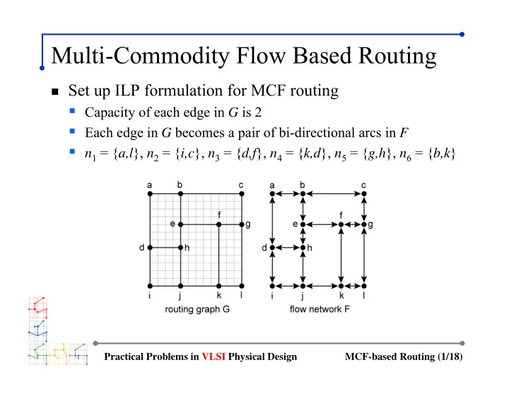
Multi-Commodity Flow Based Routing

Set up ILP formulation for MCF routing

Capacity of each edge in G is 2 Each edge in G becomes a pair of bi-directional arcs in F n1 = {a,l}, n2 = {i,c}, n3 = {d,f}, n4 = {k,d}, n5 = {g,h}, n6 = {b,k}

Practical Problems in VLSI Physical Design MCF-based Routing (2/18)

Flow Network

Each arc has a cost based on its length

Let xe

k denote a binary variable for arc e w.r.t. net k

xe

k = 1 means net k uses arc e in its route

Total number of x-variables: 16 × 2 × 6 = 192

Practical Problems in VLSI Physical Design MCF-based Routing (3/18)

ILP Objective Function

Minimize

Practical Problems in VLSI Physical Design MCF-based Routing (4/18)

ILP Demand Constraint

Utilize demand constant

zv

k = 1 means node v is the source of net k (= −1 if sink)

Total number of z-constants: 12 × 6 = 72

Practical Problems in VLSI Physical Design MCF-based Routing (5/18)

ILP Demand Constraint (cont)

Node a: source of net n1

Practical Problems in VLSI Physical Design MCF-based Routing (6/18)

ILP Demand Constraint (cont)

Node b: source of net n6

Practical Problems in VLSI Physical Design MCF-based Routing (7/18)

ILP Capacity Constraint

Each edge in the routing graph allows 2 nets

Practical Problems in VLSI Physical Design MCF-based Routing (8/18)

ILP Solutions

Min-cost: 108 (= sum of WL), 22 non-zero variable

Practical Problems in VLSI Physical Design MCF-based Routing (9/18)

ILP-based MCF Routing Solution

Net 6 is non-optimal

Due to congestion

Practical Problems in VLSI Physical Design MCF-based Routing (10/18)

Drawback of ILP-based Method

ILP is non-scalable

Runtime quickly increases with bigger problem instances

Shragowitz and Keel presented a heuristic instead

Called MM (MiniMax) heuristic [1987] Repeatedly perform shortest path computation and rip-up-and-

reroute

Practical Problems in VLSI Physical Design MCF-based Routing (11/18)

MM Heuristic

Initial set up: shortest path computation

Ignore capacity, some paths are not unique

Practical Problems in VLSI Physical Design MCF-based Routing (12/18)

First Iteration of MM Heuristic

Step 1

Capacity of channel c(e,f) and c(d,i) is violated Max overflow M1 = 3 − 2 = 1 > 0, so we proceed Notation: channel c(e,f) represents arc pair (e,f) and (f,e)

Practical Problems in VLSI Physical Design MCF-based Routing (13/18)

First Iteration of MM Heuristic (cont)

Step 2

Set of channels with overflow of M1: J1 = {c(d,i), c(e,f)} Set of channels with overflow of M1 and M1 − 1 : J1

0 = {c(a,d),

c(e,h), c(i,j), c(j,k), c(d,i), c(e,f)}

Step 3

Cost of J1

0 = {c(a,d), c(e,h), c(i,j), c(j,k), c(d,i), c(e,f)} is ∞

Practical Problems in VLSI Physical Design MCF-based Routing (14/18)

First Iteration of MM Heuristic (cont)

Step 4

Set of nets using channels in J1: K1 = {n1, n2, n3, n4, n5, n6} Set of nets using channels in J1

0: K1 0 = K1

Practical Problems in VLSI Physical Design MCF-based Routing (15/18)

First Iteration of MM Heuristic (cont)

Step 5

Compute shortest paths for nets in K1 using new cost (= Step 3) n1 & n6 have non-infinity cost, so we proceed

Practical Problems in VLSI Physical Design MCF-based Routing (16/18)

First Iteration of MM Heuristic (cont)

Step 6

Net with minimum wirelength increase between n1 & n6: k0 = n1

Practical Problems in VLSI Physical Design MCF-based Routing (17/18)

First Iteration of MM Heuristic (cont)

Step 7

Use new routing for n1 Wirelength didn’t change, but congestion improved

Practical Problems in VLSI Physical Design MCF-based Routing (18/18)

Second Iteration of MM Heuristic

Details in the book

Use new routing for n3 Wirelength increased (due to detour in n3), but congestion

improved