Mul.scale bo3om-up simula.ons of charge and energy transport - - PowerPoint PPT Presentation

Björn ¡Baumeier ¡

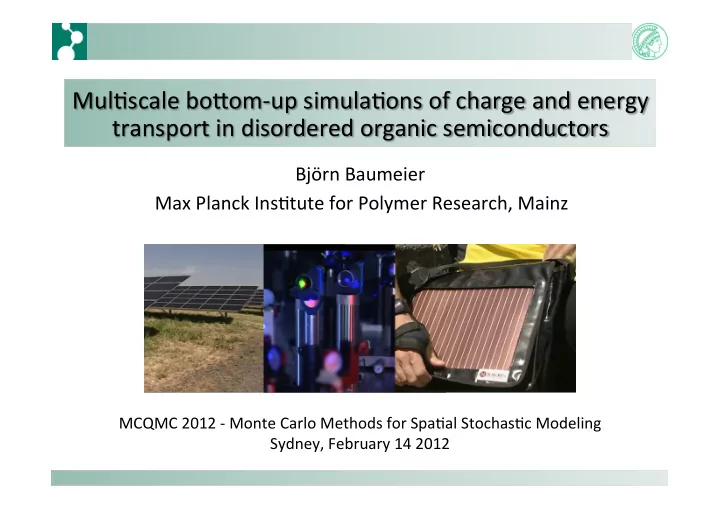
Mul.scale ¡bo3om-­‑up ¡simula.ons ¡of ¡charge ¡and ¡energy ¡ transport ¡in ¡disordered ¡organic ¡semiconductors ¡

Max ¡Planck ¡Ins.tute ¡for ¡Polymer ¡Research, ¡Mainz ¡

MCQMC ¡2012 ¡-­‑ ¡Monte ¡Carlo ¡Methods ¡for ¡Spa.al ¡Stochas.c ¡Modeling ¡ Sydney, ¡February ¡14 ¡2012 ¡

Group ¡ Denis ¡Andrienko ¡

• V. ¡Rühle ¡(Cambridge) ¡
• A. ¡Lukyanov ¡(D-­‑Fine) ¡
• T. ¡Vehoff ¡ ¡(VDI-­‑TZ) ¡
• F. ¡May ¡ ¡
• M. ¡Schrader ¡ ¡
• P. ¡Kordt ¡
• C. ¡Poelking ¡

¡ Collaborators ¡

• J. ¡Kirkpatrick ¡(Oxford) ¡
• J. ¡Nelson ¡(IC ¡London) ¡
• C. ¡Lennartz ¡(BASF) ¡

¡ Funding ¡ German-­‑Korean ¡IRTG ¡ ¡ BMBF ¡MESOMERIE ¡ SPP ¡1355 ¡

Acknowledgments ¡

Outline ¡

• 1. Compound ¡design ¡in ¡organic ¡electronics ¡

– fundamentals, ¡aims, ¡and ¡limita.ons ¡ – photoelectric ¡processes ¡in ¡organic ¡photovoltaic ¡cells ¡

• 2. Mul.scale ¡workflow ¡for ¡microscopic ¡charge ¡transport ¡simula.ons ¡

– mul.scale ¡“challenge” ¡ – Ménage ¡à ¡trois: ¡ ¡density-­‑func.onal ¡theory, ¡classical ¡Molecular ¡Dynamics, ¡ ¡kine.c ¡Monte-­‑Carlo ¡ ¡ ¡

• 3. Stochas.c ¡Graph ¡Model ¡with ¡Weighted ¡Edges ¡

1. Stochas.c ¡model ¡of ¡ver.ces ¡(hopping ¡sites) ¡ 2. Stochas.c ¡model ¡of ¡edges ¡(connected ¡hopping ¡sites) ¡ 3. Weigh.ng ¡of ¡edges ¡

1. Simula.on ¡of ¡correlated ¡site ¡energies ¡ 2. Simula.on ¡of ¡transfer ¡integral ¡

• 4. Outlook ¡

Organic ¡Electronics ¡

h3p://dvice.com/pics/ge_oledsfront.jpg ¡

¡ Organic ¡Light ¡Emi8ng ¡Diodes ¡ Organic ¡Photovoltaic ¡Cells ¡ solu%on ¡processability ¡

• spin-­‑coa.ng ¡ ¡
• inkjet-­‑prin.ng ¡

tunability ¡

• electronic ¡structure ¡(charge ¡

transport, ¡op.cal ¡proper.es) ¡

• morphology ¡control ¡(crystalliza.on, ¡

self-­‑assembly) ¡via ¡side ¡groups ¡ development ¡

• life ¡.me ¡of ¡OLEDs ¡
• efficiency ¡of ¡OPV ¡cells ¡

structure-­‑processing-­‑property ¡rela.onships ¡for ¡ “ra.onal ¡compound ¡design” ¡

Relevant ¡photoelectric ¡processes ¡in ¡OPV ¡

(1) ¡ (2) ¡ (3) ¡ (4) ¡ (1) ¡Exciton ¡formaEon ¡ ¡absorp.on ¡proper.es ¡of ¡materials ¡ ¡ (2) Exciton ¡diffusion ¡ ¡migra.on ¡of ¡local ¡excitons ¡ (3) ¡Exciton ¡separaEon ¡ ¡charge ¡transfer ¡excitons ¡at ¡interface ¡ ¡ (4) Charge ¡carrier ¡dynamics ¡ ¡transport ¡of ¡free ¡charges ¡ [+ ¡geminate/non-­‑geminate ¡recombina.on] ¡

Compound ¡design: ¡experiments ¡

NMR, ¡WAXS: ¡averaged ¡quan..es, ¡no ¡distribu.on ¡func.ons ¡ Is ¡the ¡improvement ¡due ¡to ¡electronic ¡structure ¡or ¡morphology? ¡

Theore.cal ¡Challenges ¡

• a. ¡Large-­‑scale ¡morphology ¡(topology ¡of ¡the ¡charge ¡percola.ng ¡network) ¡
• b. ¡Local ¡mutual ¡orienta.ons/posi.ons ¡of ¡molecules ¡
• c. ¡Electronic ¡structure ¡(reorganiza.on ¡energy, ¡driving ¡force, ¡electronic ¡coupling) ¡

Workflow ¡of ¡charge ¡transport ¡simula.ons ¡

ωij = J2

ij

~ r π λijkBT exp " −(∆Eij − λij)2 4λijkBT #

Marcus ¡type ¡hopping ¡rate: ¡

Current filaments Force field Electrostatics and polarization Atomistic morphology Master equation Electronic coupling

driving forces partial charges energy scans charge mobility polarizabilities transport dynamics

ϕ

• µi

qi i j ωij Jij

Sopware ¡

votca.org ¡ C++, ¡scrip.ng, ¡test ¡suite, ¡hg, ¡wiki ¡pages, ¡bug ¡tracker ¡

Versa.le ¡Object-­‑oriented ¡Toolkit ¡for ¡Coarse-­‑graining ¡Applica.ons ¡

ARTICLE pubs.acs.org/JCTC

Microscopic Simulations of Charge Transport in Disordered Organic Semiconductors

Victor R€ uhle,† Alexander Lukyanov,† Falk May,† Manuel Schrader,† Thorsten Vehoff,† James Kirkpatrick,‡ Bj€

• rn Baumeier,†,§ and Denis Andrienko*,†,§,||

†Max Planck Institute for Polymer Research, Ackermannweg 10, 55128 Mainz, Germany ‡Oxford Centre for Collaborative Applied Mathematics (OCCAM), University of Oxford, St Giles’ 24-29, OX1 3LB Oxford,

United Kingdom

§Institute for Pure and Applied Mathematics, University of California Los Angeles, 460 Portola Plaza, Los Angeles, California 90095,

United States

)

Center for Organic Photonics and Electronics and School of Chemistry and Biochemistry, Georgia Institute of Technology, Atlanta, Georgia 30332, United States

b

S Supporting Information

ABSTRACT: Charge carrier dynamics in an organic semiconductor can often be described in terms of charge hopping between localized states. The hopping rates depend on electronic coupling elements, reorganization energies, and driving forces, which vary as a function of position and orientation of the molecules. The exact evaluation of these contributions in a molecular assembly is computationally prohibitive. Various, often semiempirical, approximations are employed instead. In this work, we review some of these approaches and introduce a software toolkit which implements them. The purpose of the toolkit is to simplify the workflow for charge transport simulations, provide a uniform error control for the methods and a flexible platform for their development, and eventually allow in silico prescreening of organic semiconductors for specific applications. All implemented methods are illustrated by studying charge transport in amorphous films of tris-(8-hydroxyquinoline)aluminum, a common organic semiconductor.

Tris(8-­‑hydroxyquinolinato)aluminium ¡(Alq3) ¡

Tris(8-­‑hydroxyquinolinato)aluminium ¡

Hole ¡reorganiza.on ¡energy: ¡0.23 ¡eV ¡ Dipole ¡moment: ¡4 ¡Debye ¡ Changes ¡the ¡direc.on ¡in ¡ions ¡ Phase: ¡amorphous ¡ Isomer: ¡meridional ¡ Green ¡light ¡emi3er ¡ Hole ¡and ¡electron ¡conductor ¡ Pronounced ¡Poole-­‑Frenkel ¡behavior ¡

• J. ¡J. ¡Kwiatkowski, ¡J. ¡Nelson, ¡H. ¡Li ¡and ¡J. ¡L. ¡Bredas, ¡W. ¡Wenzel, ¡and ¡C. ¡Lennartz, ¡

Simula(ng ¡charge ¡transport ¡in ¡tris(8-­‑hydroxyquinoline) ¡aluminium ¡(Alq3), ¡

• Phys. ¡Chem. ¡Chem. ¡Phys. ¡10, ¡1852, ¡2008 ¡

Yuki ¡Nagata ¡and ¡Chris.an ¡Lennartz ¡ Atomis(c ¡simula(on ¡on ¡charge ¡mobility ¡of ¡amorphous ¡tris(8-­‑hydroxyquinoline) ¡ aluminum ¡(Alq3): ¡Origin ¡of ¡Poole-­‑Frenkel-­‑type ¡behavior, ¡

• J. ¡Chem. ¡Phys. ¡129, ¡034709, ¡2008 ¡

Box ¡of ¡512 ¡molecules ¡ experiment ¡

• A. ¡Lukyanov, ¡C. ¡Lennartz, ¡D. ¡Andrienko, ¡Phys. ¡Stat. ¡Sol. ¡A, ¡2009 ¡

Alq3: ¡Force ¡Field ¡and ¡Morphology ¡

21 ¡unknown ¡angle ¡and ¡dihedral ¡ ¡poten.als ¡ ¡ ¡ ¡ ¡[scans ¡and ¡fits ¡using ¡B3LYP/6-­‑311+g(d,p)] ¡ par.al ¡charges ¡-­‑ ¡CHELPG ¡ van ¡der ¡Waals ¡parameters ¡– ¡OPLSaa ¡ Ligands ¡-­‑ ¡rigid ¡

ρ = 1.5 g/cm3

Tg = 448 K

−14 −12 −10 −8 −6 −4 −2

log[(JZINDO/eV)2]

−14 −12 −10 −8 −6 −4 −2

log[(JDFT/eV)2]

50 100 50 100

• depend ¡on ¡posi.ons, ¡
• rienta.ons ¡
• distribu.ons ¡are ¡not ¡Gaussian ¡
• span ¡several ¡orders ¡of ¡

magnitude ¡

• semiempirical ¡and ¡DFT ¡methods ¡

agree ¡

Alq3: ¡Electronic ¡coupling ¡elements ¡

ZINDO: ¡ ¡J. ¡Kirkpatrick, ¡ ¡Int. ¡J. ¡Quantum ¡Chem. ¡108, ¡51 ¡(2008) ¡ DFT: ¡ ¡E. ¡F. ¡Valeev, ¡V. ¡Coropceanu, ¡D. ¡A. ¡da ¡Silva ¡Filho, ¡S. ¡Salman, ¡J.-­‑L. ¡Bredas, ¡J. ¡Am. ¡Chem. ¡Soc. ¡128, ¡9882 ¡(2006) ¡ ¡B. ¡Baumeier, ¡J. ¡Kirkpatrick, ¡D. ¡Andrienko, ¡Phys. ¡Chem. ¡Chem. ¡Phys. ¡12, ¡11103 ¡(2010) ¡

Jij = hφi| ˆ H|φji φij

• ­‑ ¡fron.er ¡orbitals ¡

ˆ H

• ­‑ ¡dimer ¡Hamiltonian ¡

Transfer ¡integrals ¡= ¡connec.vity ¡

• transfer ¡integrals ¡reflect ¡topological ¡

connec.vity ¡in ¡the ¡system ¡

• energe.c ¡disorder ¡weights ¡the ¡

“quality” ¡of ¡the ¡connec.on ¡

Site ¡energy: ¡electrosta.cs ¡and ¡polariza.on ¡

5 ¡neighbors ¡ 6 ¡neighbors ¡

Screening: ¡Y. ¡Nagata, ¡C. ¡Lennartz, ¡J. ¡Chem. ¡Phys. ¡2008, ¡129, ¡034709. ¡ Thole ¡model: ¡B. ¡Thole, ¡Chem. ¡Phys. ¡1981, ¡59, ¡341–350. ¡

Eel

i =

1 4⇡✏0 X

ai

X

bk k6=i

• qc

ai − qn ai

• qn

bk

✏sraibk ✏(r) = ✏∞ − (✏∞ − 1) ✓ 1 + sr + 1 2s2r2 ◆ e−sr ~ µ(k+1)

ai

= ! ~ F (k)

ai ↵ai + (1 − !)~

µ(k)

ai

Coulomb ¡interacEon ¡(with ¡bulk ¡screening) ¡ Phenomenological ¡distance-­‑dependence ¡ Explicit ¡polarizaEon ¡via ¡polarizable ¡force-­‑fields ¡

Master ¡Equa.on ¡

mapping ¡

Site-­‑occupa.on ¡based ¡descrip.on ¡ ¡

mean-­‑field ¡

State-­‑based ¡descrip.on ¡ ¡

state-­‑to-­‑site: ¡ ¡J. ¡Co3aar, ¡P.A. ¡Bobbert, ¡Phys. ¡Rev. ¡B ¡74, ¡115204 ¡(2006). ¡ kmc: ¡ ¡A.P.J. ¡Jansen, ¡An ¡Introduc.on ¡To ¡Monte ¡Carlo ¡Simula.ons ¡Of ¡Surface ¡Reac.ons, ¡cond-­‑mat/0303028 ¡

∂Pα ∂t = X

β

PβΩβα − X

β

PαΩαβ Pα -­‑ ¡occupa.on ¡probability ¡of ¡a ¡state ¡ ¡ ∂pi ∂t = X

j

pj(1 − pi)ωji − pi(1 − pj)ωij pi -­‑ ¡occupa.on ¡probability ¡of ¡a ¡site ¡

ωij

Kine.c ¡Monte ¡Carlo ¡

KMC ¡explicitly ¡simulates ¡the ¡ dynamics ¡of ¡charge ¡carriers ¡by ¡ construc.ng ¡a ¡Markov ¡chain ¡in ¡ state ¡space. ¡ ¡ ¡ Can ¡find ¡both ¡sta.onary ¡and ¡ transient ¡solu.ons ¡of ¡the ¡ master ¡equa.on. ¡ ¡ Only ¡states ¡with ¡a ¡direct ¡link ¡to ¡ the ¡current ¡state ¡are ¡needed ¡at ¡ each ¡step. ¡ ¡ ¡ Extensions ¡to ¡mul.ple ¡charge ¡ carriers ¡(without ¡the ¡mean-­‑field ¡ approxima.on), ¡site-­‑

• ccupa.on ¡

dependent ¡rates, ¡and ¡different ¡ types ¡of ¡interac.ng ¡par.cles ¡ and ¡processes, ¡are ¡

• straighzorward. ¡

Alq3: ¡Poole-­‑Frenkel ¡plot ¡

Energe.c ¡disorder ¡reduces ¡the ¡ value ¡of ¡mobility ¡by ¡six ¡orders ¡of ¡

• magnitude. ¡ ¡

¡ The ¡Poole-­‑Frenkel ¡behavior ¡for ¡ small ¡fields ¡can ¡only ¡be ¡observed ¡ if ¡correlated ¡disorder ¡is ¡taken ¡into ¡

• account. ¡ ¡

¡ For ¡a ¡system ¡with ¡such ¡large ¡ energe.c ¡disorder ¡the ¡absolute ¡ values ¡of ¡(non-­‑dispersive) ¡ mobility ¡are ¡systema.cally ¡

• veres.mated ¡due ¡to ¡significant ¡

finite ¡size ¡effects ¡

h~ vi = X

i,j

pj!ji(~ ri ~ rj) = ˆ µ~ F

0.010 0.015 0.020 0.025

µ (cm2/Vs)

no disorder 300 400 500 600 700 800 900 1000

F 1/2 (V/cm)1/2

10−9 10−8 10−7

µ (cm2/Vs)

uncorrelated disorder correlated disorder

Alq3: ¡Occupa.on ¡probabili.es ¡and ¡currents ¡

• ccupa.on ¡probabili.es ¡

4096 ¡molecules ¡ current ¡filaments ¡ 512 ¡molecules ¡ All ¡sites ¡are ¡sampled ¡(can ¡be ¡also ¡checked ¡using ¡detailed ¡balance) ¡ Currents ¡have ¡preferred ¡pathways ¡(correlated ¡disorder) ¡– ¡current ¡filaments ¡

current ¡filaments: ¡ ¡J.J.M. ¡van ¡der ¡Holst, ¡ ¡M.A. ¡Uij3ewaal, ¡B. ¡Ramachandhran, ¡R. ¡Coehoorn, ¡P.A. ¡Bobbert, ¡G.A. ¡de ¡Wijs, ¡R.A. ¡de ¡Groot, ¡

• Phys. ¡Rev. ¡B ¡79, ¡085203 ¡(2009). ¡

finite ¡size ¡effects: ¡A. ¡Lukyanov, ¡D. ¡Andrienko, ¡Phys. ¡Rev. ¡B, ¡2010 ¡

Mobility ¡does ¡not ¡converge ¡with ¡the ¡increase ¡of ¡the ¡box ¡size? ¡

Boxes ¡of ¡molecules ¡ ¡ 512 ¡= ¡8 ¡× ¡8 ¡× ¡8 ¡ 2197 ¡= ¡13 ¡× ¡13 ¡× ¡13 ¡ 4096 ¡= ¡16 ¡× ¡16 ¡× ¡16 ¡ 13824 ¡= ¡24 ¡× ¡24 ¡× ¡24 ¡

Alq3: ¡Finite ¡size ¡effects ¡

10,000 ¡molecules ¡max ¡(ZINDO ¡level) ¡ 30 ¡× ¡30 ¡× ¡30 ¡la|ce ¡ ¡ Sampling ¡of ¡full ¡DOS ¡is ¡not ¡possible ¡ Mean ¡energy ¡of ¡a ¡charge ¡carrier ¡ Dispersive ¡to ¡non-­‑dispersive ¡transport ¡

• A. ¡Lukyanov, ¡D. ¡Andrienko, ¡Phys. ¡Rev. ¡B, ¡2010 ¡

Dispersive ¡versus ¡non-­‑dispersive ¡transport ¡

EN = * Z−1

N N

X

n=1

✏ne−✏n +

✏n -­‑ ¡Gaussian ¡distributed ¡

E∞/σ = −σ/kBT

(σ/kBT)2 = −5.7 + 1.05lnN

σ/kBT = 5.4

Advantages ¡and ¡Limita.ons ¡

bulk ¡heterojuncEon ¡ Domains ¡~ ¡10nm ¡ Device ¡> ¡100nm ¡ ü parameter-­‑free ¡direct ¡link ¡between ¡chemical ¡structure, ¡processing, ¡and ¡property ¡ ü allows ¡microscopic ¡understanding ¡of ¡the ¡fundamental ¡physical ¡processes ¡ ü formula.on ¡of ¡design ¡rules ¡ ⚡ computa.onally ¡extremely ¡demanding ¡ ⚡ treatable ¡system ¡sizes ¡limited ¡to ¡15-­‑20nm ¡length ¡(10000 ¡molecules) ¡ ⚡ systema.c ¡dependence ¡of ¡mobility ¡on ¡system ¡size ¡ wait ¡for ¡bigger/faster ¡ computers? ¡ StochasEc ¡modeling! ¡ Volker ¡Schmidt ¡ Ole ¡Stenzel ¡

Stochas.c ¡model ¡of ¡ver.ces ¡(hopping ¡sites) ¡

Original ¡

• Hopping ¡sites ¡generated ¡by ¡microscopic ¡

model ¡are ¡interpreted ¡as ¡realiza.on ¡of ¡ point-­‑process ¡model ¡

• Rather ¡regular, ¡but ¡s.ll ¡random ¡structure ¡ ¡
• No ¡clustering ¡of ¡points ¡
• g(r) ¡propor.onal ¡to ¡the ¡rela.ve ¡frequency ¡
• f ¡point ¡pairs ¡with ¡distance ¡r ¡ ¡
• Hard-­‑core ¡distance ¡(minimum ¡distance) ¡

between ¡points, ¡since ¡g(r) ¡= ¡0 ¡for ¡0 ¡< ¡r ¡< ¡ 0.6nm ¡

• Rather ¡regular ¡point ¡process, ¡since ¡has ¡
• nly ¡three ¡(narrow) ¡oscilla.ons. ¡

Stochas.c ¡point-­‑process ¡model: ¡Itera.ve ¡sop-­‑core ¡model ¡

• Goal: ¡Simula.on ¡of ¡point ¡process ¡with ¡high ¡intensity ¡and ¡large ¡distances ¡ ¡
• Sop-­‑core ¡model ¡

– Step ¡1: ¡Homogeneous ¡Poisson ¡ ¡ point ¡process. ¡No ¡interac.on ¡of ¡points ¡ – Step ¡2: ¡Each ¡point ¡ ¡ ¡ ¡ ¡ ¡ ¡is ¡assigned ¡a ¡ ¡ random ¡radius ¡ ¡ ¡ ¡ ¡ ¡ ¡ ¡ ¡ ¡ ¡ ¡, ¡where ¡ ¡ ¡ ¡ ¡ ¡is ¡a ¡ con.nuous ¡distribu.on ¡func.on ¡on ¡ ¡ – Steps ¡3 ¡& ¡4: ¡Delete ¡all ¡points ¡that ¡are ¡ ¡ contained ¡in ¡a ¡larger ¡sphere ¡ – Finally: ¡Each ¡point ¡ ¡ ¡ ¡ ¡has ¡a ¡distance ¡to ¡ its ¡nearest ¡neighbor ¡point ¡larger ¡than ¡ – Maximum ¡intensity ¡(average ¡number ¡of ¡ points ¡per ¡unit ¡volume) ¡of ¡sop-­‑core ¡ ¡ process ¡is ¡limited. ¡

• Therefore: ¡itera.ve ¡sop-­‑core ¡model ¡

n

S

F Rn ~

F ) , [ ∞

n

S

n

R

Stochas.c ¡point-­‑process ¡model: ¡Itera.ve ¡sop-­‑core ¡model ¡

• Itera.ve ¡sop-­‑core ¡model ¡

– Step ¡1: ¡sop-­‑core ¡model ¡ ¡ – Step ¡2: ¡second, ¡independent ¡realiza.on ¡

• f ¡a ¡sop-­‑core ¡process ¡in ¡the ¡

complementary ¡phase ¡(blue ¡circles). ¡ ¡ – Step ¡3 ¡& ¡4: ¡delete ¡all ¡points ¡that ¡interfere ¡ with ¡previous ¡realiza.on ¡ – Step ¡5: ¡repeat ¡steps ¡2-­‑4 ¡un.l ¡desired ¡ intensity ¡is ¡reached ¡ – Finally: ¡Only ¡consider ¡points ¡(without ¡the ¡ radii) ¡

Model ¡valida.on ¡

Hopping ¡sites ¡by ¡microscopic ¡model ¡ Hopping ¡sites ¡by ¡point-­‑process ¡model ¡

Model ¡valida.on ¡

pair-­‑correla.on ¡func.on ¡ nearest-­‑neighbor-­‑distance ¡ distribu.on ¡func.on ¡ spherical ¡contact ¡ ¡ distribu.on ¡func.on ¡

• Comparing ¡structural ¡characteris.cs ¡for ¡the ¡configura.on ¡of ¡hopping ¡sites ¡generated ¡

by ¡microscopic ¡model ¡and ¡by ¡itera.ve ¡sop-­‑core ¡model ¡

• Excellent ¡agreement ¡

Black: ¡ ¡microscopic ¡model ¡ Red: ¡ ¡itera.ve ¡sop-­‑core ¡model ¡

Stochas.c ¡graph ¡model: ¡connec.ng ¡ver.ces ¡

Points ¡ ¡ ¡ ¡ ¡ ¡and ¡ ¡ ¡ ¡ ¡ ¡are ¡connected ¡ according ¡to ¡a ¡Bernoulli ¡experiment, ¡ with ¡probability ¡ ¡ ¡ ¡ ¡depending ¡on ¡ their ¡distance. ¡ Black: ¡ ¡microscopic ¡model ¡ Red: ¡ ¡fi3ed ¡func.on ¡ Probability ¡of ¡two ¡hopping ¡sites ¡ being ¡connected ¡

i

S

j

S p

Microscopic ¡model ¡ StochasEc ¡graph ¡model ¡

Model ¡of ¡correlated ¡site-­‑energies: ¡Moving-­‑average ¡approach ¡

• Edge ¡weight ¡is ¡given ¡by ¡

¡

• Site ¡energies ¡ ¡ ¡ ¡ ¡ ¡ ¡ ¡ ¡ ¡ ¡ ¡ ¡are ¡normally ¡distributed ¡ ¡

¡ ¡ ¡ ¡ ¡ ¡ ¡ ¡ ¡ ¡ ¡ ¡ ¡ ¡ ¡ ¡ ¡ ¡ ¡ ¡ ¡ ¡, ¡but ¡have ¡a ¡spa.al ¡correla.on ¡

( )

⎟ ⎟ ⎠ ⎞ ⎜ ⎜ ⎝ ⎛ − Δ − = T k E T k J h

B ij ij ij B ij ij

λ λ π π ω 4 exp 4 2

2 2 j i E

E ,

( )

2

, ~ σ µ N Ei

• Every ¡point ¡is ¡ ¡ ¡ ¡ ¡ ¡ ¡assigned ¡the ¡triple ¡ ¡ ¡ ¡ ¡ ¡ ¡ ¡ ¡ ¡ ¡ ¡ ¡ ¡ ¡ ¡ ¡ ¡ ¡ ¡ ¡ ¡, ¡where ¡

¡ ¡ ¡ ¡ ¡ ¡ ¡ ¡ ¡ ¡ ¡ ¡ ¡ ¡ ¡ ¡ ¡ ¡ ¡ ¡ ¡ ¡ ¡ ¡ ¡ ¡ ¡ ¡ ¡ ¡ ¡ ¡ ¡ ¡ ¡ ¡ ¡ ¡ ¡ ¡ ¡ ¡ ¡ ¡ ¡ ¡ ¡ ¡ ¡ ¡ ¡ ¡ ¡ ¡ ¡ ¡ ¡ ¡ ¡ ¡ ¡ ¡ ¡ ¡ ¡ ¡ ¡ ¡ ¡ ¡ ¡ ¡ ¡ ¡ ¡ ¡ ¡ ¡ ¡ ¡ ¡ ¡ ¡ ¡ ¡ ¡and ¡ ¡ ¡ ¡ ¡ ¡ ¡ ¡ ¡ ¡ ¡ ¡ ¡ ¡ ¡ ¡ ¡ ¡ ¡ ¡ ¡ ¡ ¡ ¡ ¡ ¡ ¡ ¡ ¡ ¡ ¡ ¡for ¡some ¡

• For ¡every ¡point ¡ ¡ ¡ ¡ ¡, ¡let ¡

¡be ¡its ¡ ¡ ¡ ¡ ¡nearest ¡neighbors ¡with ¡corresponding ¡marks ¡ ¡ (including ¡the ¡point ¡itself) ¡

• Define ¡energy ¡ ¡ ¡ ¡ ¡(of ¡site ¡ ¡ ¡ ¡ ¡) ¡by ¡ ¡

i

S

( )

) ( ) ( ,

,

b i a i i

R R S ⎟ ⎟ ⎠ ⎞ ⎜ ⎜ ⎝ ⎛ − − ) 1 ( ), 1 ( ~

2 ) (

ω σ ω µ L L N R a

i

( )

ω σ µω

2 ) (

, ~ N R b

i

] 1 , [ , ∈ > ω L

i

S

( ) ( ) ( ) ( )

) , ( ) , ( ) ( ) , 2 ( ) , 2 ( ) 2 ( ) , 1 ( ) , 1 ( ) 1 (

, , ,..., , , , , ,

b L i a L i L i b i a i i b i a i i

R R S R R S R R S L



ed uncorrelat b i correlated L n a n i i

R R E

) ( 1 ) , (

+ =∑

=

    

i

E

i

S

Simula.on ¡of ¡transfer ¡integral ¡ ¡

• ¡Transfer ¡integral ¡ ¡ ¡ ¡ ¡ ¡depends ¡on ¡the ¡distance ¡between ¡the ¡hopping ¡sites ¡ ¡ ¡ ¡ ¡ ¡ ¡ ¡ ¡ ¡ ¡
• ¡ ¡
• ¡ ¡ ¡ ¡ ¡ ¡ ¡ ¡ ¡ ¡ ¡depend ¡on ¡the ¡distance ¡between ¡the ¡points. ¡ ¡

¡

ij

J

j i S

S , ) , ( ~ ) log(

2 2

σ µ N Jij

short ¡distances ¡ ¡ ¡ medium ¡distances ¡ ¡ large ¡distances ¡ ¡

2

,σ µ

Valida.on: ¡Example ¡of ¡fit ¡

• ¡ ¡
• ¡Es.ma.on ¡of ¡ ¡ ¡ ¡ ¡ ¡ ¡ ¡ ¡ ¡ ¡ ¡ ¡ ¡ ¡ ¡ ¡ ¡ ¡ ¡ ¡ ¡ ¡ ¡ ¡ ¡ ¡ ¡ ¡from ¡microscopic ¡model ¡
• ¡Es.ma.on ¡of ¡ ¡ ¡ ¡ ¡ ¡ ¡ ¡ ¡ ¡ ¡ ¡ ¡ ¡ ¡ ¡ ¡ ¡ ¡ ¡ ¡ ¡ ¡ ¡ ¡ ¡ ¡ ¡ ¡ ¡ ¡from ¡microscopic ¡model ¡
• ¡Fi|ng ¡of ¡parametric ¡curves ¡ ¡
• ¡Two ¡hopping ¡sites ¡with ¡distance ¡ ¡ ¡ ¡ ¡are ¡assigned ¡a ¡squared ¡transfer ¡integral ¡by ¡

¡ ¡ ¡ ¡ ¡ ¡ ¡ ¡ ¡ ¡ ¡ ¡ ¡ ¡ ¡ ¡ ¡ ¡ ¡ ¡ ¡ ¡ ¡ ¡ ¡ ¡ ¡ ¡ ¡ ¡ ¡ ¡ ¡with ¡ ¡ ¡ ¡ ¡ ¡

) distance ( µ µ = ) distance (

2 2

σ σ = ) exp(

2 ij ij

X J =

d

)) ( ), ( ( ~

2 1 1

d d N Xij σ µ

mean ¡value ¡ variance ¡

) ( ), (

2 1 1

⋅ ⋅ σ µ ) , ( ~ ) log(

2 2

σ µ N Jij

) (

1 ⋅

µ

) (

2 1 ⋅

σ

Microscopic ¡model ¡

IteraEve ¡soW-­‑core ¡model ¡ graph ¡ver(ces ¡ Bernoulli ¡model ¡ ¡ vertex ¡connec(vity ¡ Moving-­‑averages ¡ correlated ¡site ¡energies ¡ Normal ¡distribuEons ¡ transfer ¡integral ¡

300 400 500 600 700 800 900 1000 F

1/2 (V/cm) 1/2

1e-05 0.0001 0.001 µ (cm

2/Vs)

without site-energies microscopic model stochastic graph model

Stochas.c ¡graph ¡model ¡ kMC ¡

Outlook: ¡bridging ¡the ¡gap ¡ ¡

bulk ¡heterojuncEon ¡ (1) microscopic ¡simula(on ¡ Acceptor ¡material ¡ (1) microscopic ¡simula(on ¡ Donor ¡material ¡ (2) ¡stochas(c ¡simula(on ¡ Acceptor ¡material ¡ (2) ¡stochas(c ¡simula(on ¡ Donor ¡material ¡ (3) ¡dynamics ¡in ¡bulk ¡morphology ¡