Motivation Silicon-based techniques are approaching practical A - PowerPoint PPT Presentation

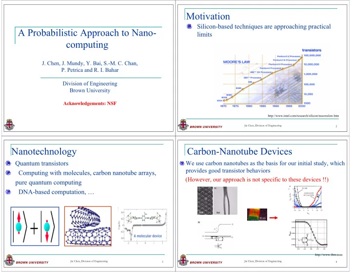
Motivation Silicon-based techniques are approaching practical A Probabilistic Approach to Nano- limits computing J. Chen, J. Mundy, Y. Bai, S.-M. C. Chan, P. Petrica and R. I. Bahar Division of Engineering Brown University Acknowledgements: NSF http://www.intel.com/research/silicon/mooreslaw.htm Jie Chen, Division of Engineering 2 BROWN UN BROWN UNIVERSITY IVERSITY Nanotechnology Carbon-Nanotube Devices Quantum transistors We use carbon nanotubes as the basis for our initial study, which provides good transistor behaviors Computing with molecules, carbon nanotube arrays, (However, our approach is not specific to these devices !!) pure quantum computing DNA-based computation, … http://www.ibm.com Jie Chen, Division of Engineering Jie Chen, Division of Engineering 3 4 BROWN UNIVERSITY BROWN UN IVERSITY BROWN UN BROWN UNIVERSITY IVERSITY

Why DNA for Self- -assembling? assembling? Why DNA for Self Non-silicon Approaches Are there other ways and other molecules that can do it Nano-scale devices are attractive but have high too? Yes, there are. probability of failure But, DNA is the best understood, plentiful, easy to Defects may fluctuate in time handle, robust, near-perfect and near-infinite specificity Cee Dekar, “Nature 2002” Jie Chen, Division of Engineering Jie Chen, Division of Engineering 5 6 BROWN UNIVERSITY BROWN UN IVERSITY BROWN UN BROWN UNIVERSITY IVERSITY Nano-architecture Approaches Our Probabilistic-based Approach “ Device failure should not cause computing systems to Nanofabrics [Goldstein-Budiu] malfunction if they have been designed from the Architecture detects faults and reconfigures beginning to tolerate faults” --- Von Neumann using redundant components Our Probabilistic-based Design Array-based approach [DeHon] “PLA” logic arrays connected by Dynamically defects tolerant conventional logic Adapts to errors as a natural consequence of probability Neural Nets [Likharev] maximization Builds neural networks from single-electron switches Removes need to actually detect Needs a training stage for proper operation faults Jie Chen, Division of Engineering Jie Chen, Division of Engineering 7 8 BROWN UN BROWN UNIVERSITY IVERSITY BROWN UNIVERSITY BROWN UN IVERSITY

Why Markov Random Fields? A Half-adder Example MRF has been widely used in pattern recognition & comm. x 0 x 2 x x x 1 2 0 Its operation does not depend on perfect devices or perfect x x 1 3 connections. x 3 MRF can express arbitrary circuits and logic operation is i x x x State i x x x State 0 1 2 0 1 3 achieved by maximizing state probability. 0 0 0 0 Valid 0 0 0 0 Valid or 1 0 0 1 Invalid 1 0 0 1 Invalid 2 0 1 0 Invalid 2 0 1 0 Valid Minimizing a form of energy that depends on neighboring 3 0 1 1 Valid 3 0 1 1 Invalid nodes in the network � low-power design s 4 1 0 0 Invalid 4 1 0 0 Valid 1 n Neighborhood of S i 5 1 0 1 Valid 5 1 0 1 Invalid − ∑ 1 st Order Clique 1 N 1 ( ) i U s 6 1 1 0 Valid 6 1 1 0 Invalid c Ν = s T ( | ) 2 P s e ∈ n c C 7 1 1 1 Invalid 7 1 1 1 Valid s i i i Z (a) For Summation (b) For Carrier 2 nd Order Clique s 3 n Jie Chen, Division of Engineering Jie Chen, Division of Engineering 9 10 BROWN UNIVERSITY BROWN UN IVERSITY BROWN UNIVERSITY BROWN UN IVERSITY Rules to Formulate Clique Energy Clique Energy for the Summation Sum over the valid states (000, 011, 101, 110) Clique energy is the negative sum of all valid states: = − + + + − − − + 1 2 2 2 4 U x x x x x x x x x x x x 0 1 2 0 1 0 2 1 2 0 1 2 ∑ = − = ( , , ) ( , , ), where 1 U x x x f x x x f x0 x1 x2 U 0 1 2 0 1 2 i i i 0 0 0 -1 We use Boolean ring conversion to express each minterm Lemma: The energy of correct 0 0 1 0 representing a valid state (i.e. ‘000’): logic state is always less than 0 1 0 0 = − − − ' ' ' (1 )(1 )(1 ) x x x x x x 0 1 2 0 1 2 that of invalid logic state by a 0 1 1 -1 = − − − − (1 )(1 ) x x x x x constant. 1 0 0 0 0 1 0 1 2 = − − − + + + − 1 x x x x x x x x x x x x 1 0 1 -1 0 1 2 0 1 0 2 1 2 0 1 2 1 1 0 -1 1 1 1 0 Jie Chen, Division of Engineering Jie Chen, Division of Engineering 11 12 BROWN UN BROWN UNIVERSITY IVERSITY BROWN UN BROWN UNIVERSITY IVERSITY

Structural and Signal Errors Take Device Errors into Design Our implementation does not distinguish between devices and connections. Sum over the valid states (000, 011, 101, 110) = − + + + − − − + Instead, we have structural-based and signal-based faults. 1 2 2 2 4 U x x x x x x x x x x x x 0 1 2 0 1 0 2 1 2 0 1 2 -- Structural-based error: Nano-scale devices contain a large number of defects or structural errors, which fluctuate on time If we take the device error into consideration, the energy scales comparable to the computation cycle. can be rewritten as: The error will result in variation in the clique = − + κ + + − − 2 energy coefficients. U Ax Bx Cx Dx x 0 1 2 0 1 − + 2 2 4 Ex x Fx x Gx x x 0 2 1 2 0 1 2 -- The second type of error is directly accounted for process noise that affects the signals. In the error-free case, A=B=C=D=E=F=G=1 Jie Chen, Division of Engineering Jie Chen, Division of Engineering 13 14 BROWN UNIVERSITY BROWN UN IVERSITY BROWN UNIVERSITY BROWN UN IVERSITY Take Structural Error into Design The Inequalities for Correct Logic We have 16 inequality relations total for this function = − + κ + + − x0 x1 x2 U 2 U Ax Bx Cx Dx x 0 1 2 0 1 − − + 0 0 0 -1 2 2 4 Ex x Fx x Gx x x 0 2 1 2 0 1 2 0 0 1 0 = − + κ + − 2 U B C F 0 1 0 0 011 0 1 1 -1 = − + κ U A 100 1 0 0 0 1 0 1 -1 < U U 011 100 1 1 0 -1 1 1 1 0 Jie Chen, Division of Engineering Jie Chen, Division of Engineering 15 16 BROWN UN BROWN UNIVERSITY IVERSITY BROWN UN BROWN UNIVERSITY IVERSITY

Take Signal Errors into Design Constraints on Clique Coefficients Gibbs distribution for an inverter is: x x We obtain the following − − 1 1 ( 2 1 0 x x x x − ) 0 1 0 1 constraints on the = ( , ) P x x e T 0 1 coefficients: Z The conditional probability is: 2G>D 2F>C 2E>A 2D>B 2G>F 2F>B 2E>C 2D>A ( , ) 2G>E P x x Constraints form a polytope = 1 0 ( | ) P x x 1 0 ( ) P x High order coefficients constraints the lower order ones 0 = − + κ + + − − − + 2 2 2 4 U Ax Bx Cx Dx x Ex x Fx x Gx x x 0 1 2 0 1 0 2 1 2 0 1 2 Reliability of high order connections determine design Jie Chen, Division of Engineering Jie Chen, Division of Engineering 17 18 BROWN UNIVERSITY BROWN UN IVERSITY BROWN UNIVERSITY BROWN UN IVERSITY Tolerance to Temperature Variation Continuous Errors in Signal By taking input around ‘1’, we get marginalized We model signal noise probability: using Gaussian process − 1 ( 1) 2 = ∫ x − + σ 1 2 η 2 ( ) ( | ) σ 2 P x P x x e dx 1 1 0 0 − − σ 1 2 1 σ =sqrt(2) 1 σ =sqrt(0.2) 0.9 σ =sqrt(0.02) 2 − µ ( ) 0.8 x 1 Design choice 1 -- Inputs around “0” & “1” − 0 0.8 = σ 2 0.7 2 P e p(x‘ 1 ) probability p(x‘ 1 ) probability gaussian 0.6 πσ 2 0.6 0.5 0.4 0.4 0.3 0.2 0.2 T=0.1 0.1 T=0.25 T=0.5 0 0 −1 −0.5 0 0.5 1 −1 −0.5 0 0.5 1 x‘ 1 x‘ 1 Design choice 2 -- Inputs around “-1” & “1” Jie Chen, Division of Engineering Jie Chen, Division of Engineering 19 20 BROWN UN BROWN UNIVERSITY IVERSITY BROWN UNIVERSITY BROWN UN IVERSITY

Error Rate Calculation Signal Error in NAND Design incorrect probability Gibbs distribution for a NAND is: x a = Error rate x c 1 (2 + 1 − − − ) correct incorrect probability x x x x x x x b = ( , , ) a b c a b c P x x x e T a b c Z 0.5 0.5 0.45 0.45 The marginalized probability P(x c ) is: 0.4 0.35 0.4 0.3 Error rate Error rate 1 0.25 0.35 0.2 0.8 0.3 0.15 p(x 1 ) probability 0.1 0.6 0.25 0.05 0 0.2 0.4 0 0.5 1 1.5 2 2.5 3 3.5 4 1 1.2 1.4 1.6 1.8 2 Temperature variation (T) of Gaussian Process Standard deviation ( σ ) of Gaussian Process T=0.1 T=0.25 0.2 Proposed design favors for low T and small σ . T=0.5 0 −1 −0.5 0 0.5 1 x c Jie Chen, Division of Engineering Jie Chen, Division of Engineering 21 22 BROWN UNIVERSITY BROWN UN IVERSITY BROWN UNIVERSITY BROWN UN IVERSITY Error Rate Calculation Tolerance to Temperature Variation 0.5 T=0.1 T=0.1 0.45 1 1 T=0.25 T=0.25 T=0.5 T=0.5 0.4 T=1 T=1 T=4 T=4 0.8 0.8 0.35 p(x‘ c ) probability p(x‘ c ) probability 0.3 Error rate 0.6 0.6 0.25 0.2 0.4 0.4 0.15 0.2 0.2 0.1 x a = 1, x b = 1 0.05 x a = 0, x b = 1 0 0 −1 −0.5 0 0.5 1 −1 −0.5 0 0.5 1 0 x‘ c x‘ c 0 0.5 1 1.5 2 2.5 3 3.5 4 T Proposed design works better at low energy state. Apply inputs “11” Apply inputs “01” Jie Chen, Division of Engineering Jie Chen, Division of Engineering 23 24 BROWN UNIVERSITY BROWN UN IVERSITY BROWN UN BROWN UNIVERSITY IVERSITY