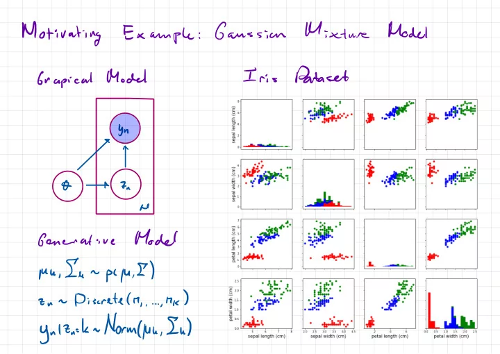
Motivating Gaussian Example : Dataset Iris Model Grapical bn - PowerPoint PPT Presentation

Mixture Model Motivating Gaussian Example : Dataset Iris Model Grapical bn O 7- a he Model Generative , In pyu ,E ) Mu - . ,hk ) Discrete ( M 2- un , . , . ynltn-kn.lt/orm4uh,Iu )

Models Motivating Hidden Mahar Example : ¢€yT Yt yi t & Za 7 z . , , ← £ Posterior Parameters t Goal : an p I O ) 10 ) ply O ly pi ) = t Can BPG do y via q intractable ply ) =/ DO = Idt PCYIO ) 7101 pcyiolplo ) pay ,

Monte Carlo Estimation Setup : Assume We graphical model probabilistic have : some x :{ 7,03 density unnormalized with A ) pcx ) ( x ) ) pay pcyix y x fdxrilxiflxl = = , x ) y = C Goal Calculate normalized density w.at expectation : . / 2- 17 Cx ) ycx ) =) :-. = /dx 2- JK ) = = [ fix ) F Enix - : : - -_ - - ,

Monte Carlo Estimators Idea ÷ Replace of integrals with samples sequences : Es ?? Ig ' fcxs ) X - Ft . S Mix ) - s I - - . . , Monte Properties Carlo estimators : are Unbiased 1 : . Es ] El F = Consistent 2 : . EKES ' lim ] o = S → as

Monte Carlo Estimators Unbiased ness : f Ks ) ) Efts Ef 's I I = = = I

# If Monte EECES Carlo Estimators Numbers Consistency Law of Large ; & fix FI is ' ) ) FT I ]= El - - 's c = = YEH It's .EE#Ef I = 's ) E lsima.IT?lEs-F53=hjzsIEIlfCxt-F5I=o

Importance Sampling Problem Often directly it not possible to is : sample from the target Xr next Xsnqcx Solution Generate from samples ) : distribution similar that proposal to ) Mk a is = fdx EIIHX ) ) fix next , MCM "X gcxi = fdx iss X S - i -

Self Importance normalized Sampling - Problem : In calculate to importance weights order evaluate to Thx 19cm need ) the ) wcx we : = IF normalized but 121×1 density text = , :-. fdxycxl calculate normally 2- 't we can Solution : Normalize Monte Carlo estimate using a 7 fax 2- next = = = = ¥ fdxycxifki F =

Self Importance normalized Sampling - Wfld Ws IZ # 17kt =p ' ) - Phil 8 ( X = 2W Unnennalized Weight Importune paly ) - is , qcxs ) ' & Es I ) s = :-. S Is s= , WS s ' f Ks I € Ews = Ws :-. S ' ' ) - flx s 5--1

Self Importance normalized Sampling - Es ÷ w1=*w ' ] ? Question ? ( F ) Es . EEE Is unbiased : i.e s.es?Ewsfk7wi--rgYyY,Es:-s?ws ' f Ks ) ) Elf 's w = = ? El ¥1 = 's E . , inequality EKD ) cel Jensen 's . K ) ) Ely when convex > y

What Proposal Optimal ? Choice of is MEhr ^ fix ) Jk ) 91×1 a - EH Variance } of Estimator Ell 'Y¥ fix ) FI ) , flat ) ' F - - - E= ( lax mail.nl/IF dxgcxi =/ " '

Default for Weighting Likelihood proposal choice : Assume Net Bayes : = fdxpiy.tl - ply ) 1×7 2- j pcylxlpcxl ply Xi = - = , [ prior Set proposal to I random not a Variable ) pcxl qcx ) = Likelihood Weights Importance : & WI pandan f Ks Is us ) = = = = .ws 's § 5--1 . ra ,

Running Mixture Model Gaussian Example . : Model Dataset Grapical Iris Yn O 7- a he Model Generative , fun pyu ,E ) Mu . ,hk ) ( M Discrete 2- un , . . , ynltn-kn.lt/orm4uh,Iu )

Problem Models Motivating Hidden Markov : §→€→ Yt yi t & Ze 7 z . , , ← It Posterior futon Goal Parameters : an fat ' Y ) PCO 't O ly , pc = a " Guess prior I likelihood " ? " Will likelihood weighty wash Cheah using a ) pcyi.it/7i:t,T Ws On 19 ) PCO ) pet ⇐ 2- ~ it ,

sample xs Manhov Chain Monte Carlo 5 1 Use - Idea to previous sample propose : x the next A of Maher Chain variables random : sequence Xl ,X5 when Markov chain ) ( discrete is time a - . . . , ... ,×s 2 xs 1×5 " " ! DX Moran property ) Xsixs " xslx is ' ( ' ' ( ) p = p Mmwov A Chain homogenous When is same trans ' ) " ) 1×5 "=×s p(Xs=×s p( '=xslX=xs X dtst . for = each s

Manha Monte Carlo Chain A Manha Convergence chain to converges : density target when ( 17 ) x a p(Xs=x lying ) n(X=× ) = . "II÷u III : 2 *¥*y¥¥± . which X=x in visited is , " frequency " with h(X=x ) J

Markov Monte Carlo Chain Balance A Markov Detailed chain homogenous : balance detailed satisfies when ' ) plxcx pix 't ' Ix ) MCX ) Mix = invariant leaves Implication ' 1×1 pcx Mix ) i /dx x ) ' ' ) 17 C Mlxspcx IX = . fdx ' I ' I ' pcxlx MCX = ' start If with sample next x a you n ' ) this then ' sample pl Mex ) and XIX XIX ~ xn

mm in Metropolis Hastings - from Starting xs sample Idea current the : mix accept proposal qcxixs ) ' generate and n a x ' xst probability with ' x = ' ) ' I 17 9 ( ( . XIX x ) ) ( I a = , qcx ' Ix , probability proposal with reject the C ) a I - "=xs the xs retain sample and previous

Metropolis Hastings - from Starting xs sample Idea current the : = mmin accept proposal qcxixs ) ' generate and ~ a × '=x xst probability with ' ' ) ' ) M q( ( XIX . X ) ) ( l a i qkllx ( × ) n probability with ( proposal reject the ) l d - "=xs xs the retain sample previous and Show Markov Exercise the that chain : balance xs ' detailed satisfies x . . .

- Hastings Balance Detailed etropolis : Balance Detailed : ' ) plxcx 't I ' Ix ) 17 C X ) Mix X = p - Hastings Metropolis Define : 8×61+09 pcxiixl - d) ( I x' Ix C ) o= = minfl.MY?,9gfIYY-j)pCx'lxlnCx ) = =

- Hastings Densities Unrormalired etropolis : Nice Can calculate property prob acceptance : ' ) from ✓ C x ) densities unhormaliced and jcx in ' ) ' I 17 ( 9 ( XIX . X ) ) ( I a mm = , qcx ' Ix × , , n s ya main ' ) ' I j ( XIX . x 9 C ) ) ( I = qcx ' Ix , xyqcx rain ' 7 ' ) X ) Cx ) ply ply X gcxlx y ) ) = , , ( I = , ' Ix pay ,

- Hastings Metropolis Choosing proposals : Sample from Mtt Independent proposers : pretor - Independent ' IX ) from a ( X pal ) = sample previous rain ' ) ' ) ply g ( x XIX ) ) , ( I a = i , qcx ' Ix pay ,× in mind ) ) ( I mm - = = , , but low Really prob simple acceptance ,

" ÷÷§\× ft large - Hastings Metropolis Choosing proposals : y Gaussian variables Continuous : f . • - ↳ - off Norm ( 82 ) ' ' ' ) qcx IX X X small or ; = , fur proposal off Trade variance - 82 small prob too good acceptance A - ; , but high correlation between samples less 82 but correlation large too : - , lower prob acceptance A Rule of ' thumb of tune I to 0.234 make 9 ,

Lecture ) Gibbs ( Next Sampling Propose Idea 1 time at variable : a , holding other variables constant ) C ply y x pix ,Xa ) ) Ix Xz = , , . x. in xi - Acceptance Ratio Car accept prob I with : = min ( ) A I = , I =

Mixture ) Gaussian ( Gibbs Sampling Lecture Next : Model Gibbs Grapical Sampler Steps E ) E ly pcznly.lu 2- µ r n , , , Y " pyu.Ely.tl Ely , 't ~ µ pcyn.IQ/uu,Iunpc/u,E , Distributions Conditional 2- 0 2- a : n he , E ) plyn.7n-h.ME ) pctn-hlyn.pe = Model Generative ' Yul - l , µ , E) 2- n=h ) pC7n=h ) µ p = , El pl7n=l ) .tk ) ? Discretely pcynl Zu - 2- - n . . . , , ynlZn=k~N0rm( Mish ) nItm-dnl9.ME Exploit ind and 2- . .