4-1. Compound Options Motivating Example: Compound options as a - PowerPoint PPT Presentation

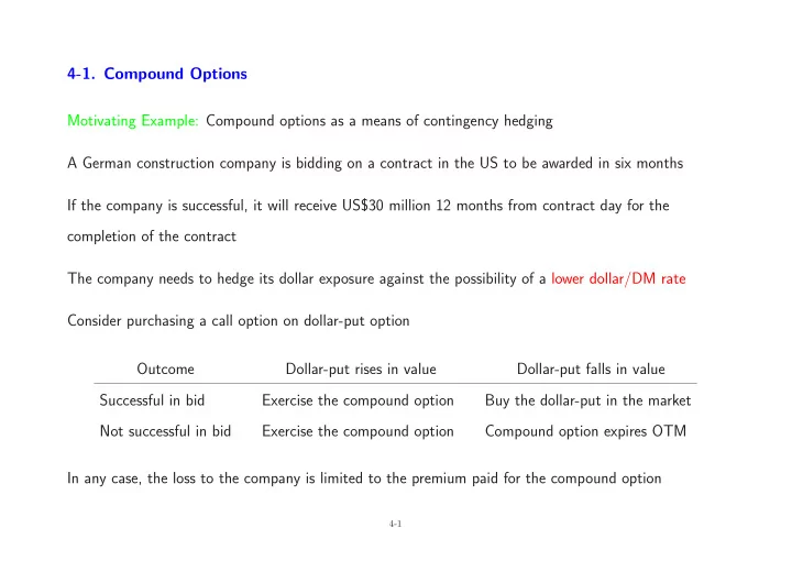
4-1. Compound Options Motivating Example: Compound options as a means of contingency hedging A German construction company is bidding on a contract in the US to be awarded in six months If the company is successful, it will receive US$30 million 12 months from contract day for the completion of the contract The company needs to hedge its dollar exposure against the possibility of a lower dollar/DM rate Consider purchasing a call option on dollar-put option Outcome Dollar-put rises in value Dollar-put falls in value Successful in bid Exercise the compound option Buy the dollar-put in the market Not successful in bid Exercise the compound option Compound option expires OTM In any case, the loss to the company is limited to the premium paid for the compound option 4-1

Motivating Example (continued) Options First payment Second payment Total premium Call on dollar-put (1) 450 points 450 points 900 points Call on dollar-put (2) 290 points 800 points 1090 points ATM vanilla put 800 points — 800 points Although more expensive than the vanilla put, the compound option offers greater flexibility and control in their application The premiums can be adjusted according to the likelihood of the company being awarded the contract A Second Example: Compound options as a means for hedging debt A liability manager wishes to hedge a portfolio of dollar floating-rate debt priced off LIBOR He seeks protection against rises in dollar interest rates over the next three years 4-2

A Second Example (continued) 1. Purchase a standard cap on three-month LIBOR for three years at a strike of 7.50% pa Cost: premium equals 2.1% of the face value of the underlying debt being hedged 2. Purchase a compound cap (“caption”) for the right to buy a cap on three-month LIBOR with a strike of 7.50% pa Cost: agreed total premium of 1.75% (for all 11 caps) and compound cap premium of 0.74% The compound cap offers a cost saving on the initial premium of a substantial amount The contingent premium would be triggered only if the cap level is breached at any three-month LIBOR fixing date and the hedger would pay the relevant agreed premium for that particular period The compound cap hedge involves a lower total cost except where interest rates rise sharply and all or most of the caps are triggered (e.g., when 9 or more caps are triggered) 4-3

Payoff: Suppose the compound option has strike K and maturity date T while the underlying option has strike K ∗ and maturity date T ∗ > T (so the underlying option lasts for T ∗ − T before expiration) There are four possible variations 1. Call on call: payoff T = max { 0 , C std ( S T , K ∗ , T ∗ − T ) − K } 2. Put on call: payoff T = max { 0 , K − C std ( S T , K ∗ , T ∗ − T ) } 3. Call on put: payoff T = max { 0 , P std ( S T , K ∗ , T ∗ − T ) − K } 4. Put on put: payoff T = max { 0 , K − P std ( S T , K ∗ , T ∗ − T ) } C std and P std are given by the Black-Scholes formula: for spot S , strike K and time to expiration τ C std ( S, K, τ ) = Se − qτ N ( d 1 ) − Ke − rτ N ( d 2 ) P std ( S, K, τ ) = Ke − rτ N ( − d 2 ) − Se − qτ N ( − d 1 ) d 2 = ln( S/K ) + ( r − q − σ 2 / 2) τ d 1 = d 2 + σ √ τ and σ √ τ 4-4

Payoff (continued) E.g., S = 100 , r = 0 . 05 , q = 0 . 03 , σ = 0 . 2 , K = 6 , T − t = 0 , K ∗ = 100 , T ∗ − T = 0 . 5 Option on a call Option on a put 20 15 15 payoff payoff 10 10 5 5 0 0 80 90 100 110 120 80 90 100 110 120 S S Call on call and call on put inherit characteristics of the underlying options while put on call and put on put have characteristics different from the underlying options 4-5

Valuation: By risk-neutral valuation, the value of a call on call is max { 0 , C std ( S T , K ∗ , T ∗ − T ) − K } C = e − r ( T − t ) E � � While an analytic expression for C is available, we first consider evaluating the integral (expectation) using a numerical integration routine (e.g., trapezoidal rule) Let f ( x ) be the PDF of the normal distribution with mean ( r − q − σ 2 / 2)( T − t ) and variance √ σ 2 ( T − t ) and apply a change of variable z = ( x − ( r − q − σ 2 / 2)( T − t )) /σ T − t � ∞ max { 0 , C std ( Se x , K ∗ , T ∗ − T ) − K } f ( x ) dx C = −∞ � ∞ � ∞ √ T − t +( r − q − σ 2 / 2)( T − t ) , K ∗ , T ∗ − T ) − K } n ( z ) dz = max { 0 , C std ( Se zσ = I ( z ) dz −∞ −∞ � ∞ � M We replace −∞ by − M (e.g., M = 6 would give a sufficiently accurate approximation), choose a large n and set h = 2 M/n to obtain � n − 1 � C ≈ h � I ( − M ) + I ( M ) + 2 I ( − M + ih ) 2 i =1 4-6

Valuation (continued) Alternatively, let S ∗ be the asset price for which C std ( S ∗ , K ∗ , T ∗ − T ) = K (e.g., S ∗ can be found using the Newton-Raphson algorithm) The compound option payoff is nonzero when S T > S ∗ (or when x > ln( S ∗ /S ) ) so � ∞ C std ( Se x , K ∗ , T ∗ − T ) − K C = e − r ( T − t ) � � f ( x ) dx ln( S ∗ /S ) Each of the three terms in the integral can be evaluated separately � ∞ Se x e − q ( T ∗ − T ) N ( d 1 ) f ( x ) dx = Se − q ( T ∗ − t ) N 2 ( D 1 , D ∗ 1. e − r ( T − t ) 1 ; ρ ) ln( S ∗ /S ) � ∞ K ∗ e − r ( T ∗ − T ) N ( d 2 ) f ( x ) dx = K ∗ e − r ( T ∗ − t ) N 2 ( D 2 , D ∗ 2. e − r ( T − t ) 2 ; ρ ) ln( S ∗ /S ) � ∞ 3. e − r ( T − t ) Kf ( x ) dx = Ke − r ( T − t ) N ( D ∗ 2 ) ln( S ∗ /S ) ( T − t ) / ( T ∗ − t ) and N 2 ( · , · ; ρ ) is the bivariate standard normal CDF with correlation � Here, ρ = coefficient ρ 4-7

Valuation (continued) The analytic pricing of the compound option relies on the following result � ∞ � µ − a bµ + c � √ f ( x ) N ( bx + c ) dx = N 2 , 1 + b 2 ν 2 ; ρ ν a √ where f ( x ) is the PDF of a N ( µ, ν 2 ) distribution and ρ = bν/ 1 + b 2 ν 2 √ 1. After completing the squares, we have µ = ( r − q + σ 2 / 2)( T − t ) and ν = σ T − t T ∗ − T and c = ln( S/K ∗ ) + ( r − q + σ 2 / 2)( T ∗ − T ) 1 Futhermore, a = ln( S ∗ /S ) , b = √ √ T ∗ − T σ σ Therefore, µ − a bµ + c ( T − t ) / ( T ∗ − t ) = D ∗ � √ 1 , 1 + b 2 ν 2 = D 1 and ρ = ν 2. Now µ = ( r − q − σ 2 / 2)( T − t ) and c = ln( S/K ∗ ) + ( r − q − σ 2 / 2)( T ∗ − T ) √ T ∗ − T σ With a, b, ν as before, we have µ − a bµ + c = D ∗ 2 and √ 1 + b 2 ν 2 = D 2 ν 4-8

Valuation (continued) 15 c c a a 10 l l l l o o n n c 10 p a u l l t p p r r 5 i i c c e e 5 0.4 0.4 110 110 0.3 0.3 100 100 Tc Tc 0.2 0.2 S S 90 90 0.1 0.1 As expected, compound calls have price characteristics and sensitivities similar to the underlying option By contrast, as the payoffs on compound puts flatten out (at close to K ) as the options become further ITM, compound puts have different price, delta, gamma and vega surfaces than the underlying options 4-9

Valuation (continued) 5 5 p p u u 4 t 4 t o o n n p 3 c 3 u a t l l p p r 2 r 2 i c i c e e 1 1 0.4 0.4 110 110 0.3 0.3 100 100 Tc Tc 0.2 0.2 S S 90 90 0.1 0.1 Hedging: Hedging compound options using the underlying options can be expensive due to higher transaction costs Hedging using the asset underlying the underlying options leads us to analyze the price sensitivities of compound options (we focus on compound puts) 4-10

Delta: The deltas of compound puts are peaked near the strike price K ∗ of the underlying option 0.3 p u t −0.1 p o u n t p 0.2 o u n t c −0.2 d a e l l l t a d 0.1 e l t a −0.3 0.4 0.4 110 110 0.3 0.3 100 100 Tc Tc 0.2 0.2 S S 90 90 0.1 0.1 Delta hedging: • Sale of a put on call is hedged by selling | ∆ | units of the underlying asset • Sale of a put on put is hedged by buying ∆ units of the underlying asset Rapid changes in ∆ as t → T means that hedging is difficult close to compound option expiration 4-11

Gamma: The gammas of compound puts can be positive or negative depending on the level of the underlying asset relative to the peaks p 0.04 u 0.04 t p o u n t p o u 0.02 n 0.02 t c g a a l m l g m 0.00 a 0.00 a m m a −0.02 0.4 0.4 110 110 0.3 0.3 100 100 Tc Tc 0.2 0.2 S S 90 90 0.1 0.1 Compound puts are high gamma instruments close to compound option expiration; elsewhere changes in asset prices do not require drastic rebalancing of the hedging portfolio 4-12

Vega: Except when the compound puts are deep OTM, increases in volatility always lead to decreases in compound option prices (negative vegas) 0 0 p −5 u p −5 t u o t n o −10 n c −10 a p l l u v t −15 e v −15 g e a g a −20 −20 −25 0.4 0.4 110 110 0.3 0.3 100 100 Tc Tc 0.2 0.2 S S 90 90 0.1 0.1 Example: T − t = 0 . 025 • Put on call: For S > 94 increases in σ leads to increases in ∆ (rapid increases around S = 100 ); for S < 94 increases in σ leads to decreases in ∆ • Put on put: Effect of σ on ∆ reversed about S = 104 4-13