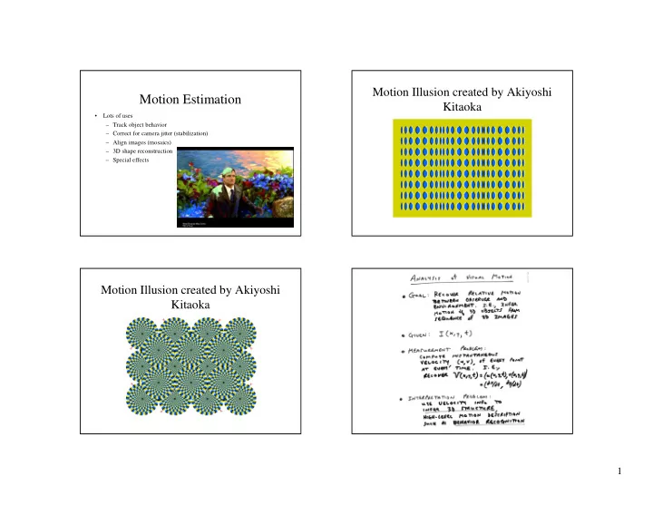
Motion Estimation Kitaoka Lots of uses Track object behavior - PowerPoint PPT Presentation

Motion Illusion created by Akiyoshi Motion Estimation Kitaoka • Lots of uses – Track object behavior – Correct for camera jitter (stabilization) – Align images (mosaics) – 3D shape reconstruction – Special effects Motion Illusion created by Akiyoshi Kitaoka 1

2

Optical flow 3

Aperture problem Aperture problem 4

5

6

Hamburg Taxi Video Hamburg Taxi Video Horn & Schunck Optical Flow 7

Fleet & Jepson Optical Flow Tian & Shah Optical Flow Solving the Aperture Problem • Basic idea: assume motion field is smooth • Horn and Schunk: add smoothness term • Lucas and Kanade: assume locally constant motion – pretend the pixel’s neighbors have the same (u,v) • If we use a 5x5 window, that gives us 25 equations per pixel! – works better in practice than Horn and Schunk 8

Lucas-Kanade Flow Lucas-Kanade Flow • Problem: more equations than unknowns • How to get more equations for a pixel? – Basic idea: impose additional constraints • Solution: solve least squares problem • most common is to assume that the flow field is smooth locally – minimum least squares solution given by solution of: • one method: pretend the pixel’s neighbors have the same (u,v) – If we use a 5x5 window, that gives us 25 equations per pixel! – The summations are over all pixels in the K x K window – This technique was first proposed by Lukas and Kanade (1981) Eigenvectors of A T A Conditions for Solvability – Optimal (u, v) satisfies Lucas-Kanade equation • Suppose (x,y) is on an edge. What is A T A? – gradients along edge all point the same direction – gradients away from edge have small magnitude When is this solvable? • A T A should be invertible – is an eigenvector with eigenvalue • A T A should not be too small due to noise – What’s the other eigenvector of A T A? – eigenvalues λ 1 and λ 2 of A T A should not be too • let N be perpendicular to small • A T A should be well-conditioned λ 1 / λ 2 should not be too large ( λ 1 = larger – • N is the second eigenvector with eigenvalue 0 eigenvalue) • The eigenvectors of A T A relate to edge direction and magnitude 9

Edge Low Texture Region – large gradients, all the same – gradients have small magnitude – large λ 1 , small λ 2 – small λ 1 , small λ 2 High Texture Region Observation • This is a two image problem BUT – Can measure sensitivity by just looking at one of the images – This tells us which pixels are easy to track, which are hard • very useful later on when we do feature tracking – gradients are different, large magnitudes – large λ 1 , large λ 2 10

Errors in Lucas-Kanade Improving Accuracy • Recall our small motion assumption • What are the potential causes of errors in this procedure? – Suppose A T A is easily invertible • This is not exact – To do better, we need to add higher order terms back – Suppose there is not much noise in the image in: • When our assumptions are violated • This is a polynomial root finding problem – Brightness constancy is not satisfied – Can solve using Newton’s method – The motion is not small • Also known as Newton-Raphson method – Lucas-Kanade method does one iteration of Newton’s method – A point does not move like its neighbors • Better results are obtained with more iterations • window size is too large • what is the ideal window size? Revisiting the Small Motion Assumption Iterative Refinement • Iterative Lucas-Kanade Algorithm 1. Estimate velocity at each pixel by solving Lucas-Kanade equations 2. Warp H towards I using the estimated flow field - use image warping techniques 3. Repeat until convergence • When is the motion small enough? – Not if it’s much larger than one pixel (2 nd order terms dominate) – How might we solve this problem? 11

Coarse-to-Fine Optical Flow Reduce the Resolution Estimation u=1.25 pixels u=2.5 pixels u=5 pixels u=10 pixels image H image H image I image I Gaussian pyramid of image H Gaussian pyramid of image I Coarse-to-Fine Optical Flow Optical Flow Result Estimation run iterative L-K warp & upsample run iterative L-K . . . image J image H image I image I Gaussian pyramid of image H Gaussian pyramid of image I 12

Spatiotemporal (x-y-t) Volumes Visual Event Detection using Volumetric Features • Y. Ke, R. Sukthankar, and M. Hebert, CMU, CVPR 2005 • Goal: Detect motion events and classify actions such as stand-up , sit-down , close-laptop , and grab-cup • Use x-y-t features of optical flow – Sum of u values in a cube – Difference of sum of v values in one cube and v values in an adjacent cube 13

3D Volumetric Features Optical Flow Features Optical flow of stand-up action (light means positive direction) Approximately 1 million features computed Classifier Action Detection • 78% - 92% detection rate on 4 action types: sit- • Cascade of binary classifiers that vote on the down , stand-up , close-laptop , grab-cup classification of the volume • 0 – 0.6 false positives per minute • Given a set of positive and negative examples at a • Note: while lengths of actions vary, the first node, each feature and its optimal threshold is frames are all aligned to a standard starting computed. Iteratively add filters at each node position for each action until a target detection rate (e.g., 100%) or false • Classifier learns that beginning of video is more discriminative than end because of variable length positive rate (e.g., 20%) is achieved • Relatively robust to viewpoint (< 45 degrees) and • Output of the node is the majority vote of the scale (< 3x) individual filters 14

Results Structure-from-Motion • Determining the 3-D structure of the world, and the motion of a camera (i.e., its extrinsic parameters) using a sequence of images taken by a moving camera – Equivalently, we can think of the world as moving and the camera as fixed • Like stereo, but the position of the camera isn’t known (and it’s more natural to use many images with little motion between them, not just two with a lot of motion) and we have a long sequence of images, not just 2 images – We may or may not assume we know the intrinsic parameters of the camera, e.g., its focal length 15

16

17

Extensions Results • Paraperspective • Look at paper figures… – [Poelman & Kanade, PAMI 97] • Sequential Factorization – [Morita & Kanade, PAMI 97] • Factorization under perspective – [Christy & Horaud, PAMI 96] – [Sturm & Triggs, ECCV 96] • Factorization with Uncertainty – [Anandan & Irani, IJCV 2002] 18

= [[e´] x F | e´] 19

Sequential Structure and Motion Sequential structure and motion Computation recovery • Initialize structure and motion from two views • For each additional view – Determine pose ������������������ ��������������������� �� � �� � ������������������ ����������������������������� – Refine and extend structure • Determine correspondences robustly by jointly estimating matches and epipolar geometry ������������� ������� �������� ����������� �������!�������� � ���������������� ��������� ��������������������"��� �"��� � ��#������� ���!� ��������� 20

Pollefeys’ Result Object Tracking • 2D or 3D motion of known object(s) • Recent survey: “Monocular model-based 3D tracking of rigid objects: A survey” available at http://www.nowpublishers.com/ 21

22

23

24