Motion Estimation Lots of uses Track object behavior Correct - - PDF document

1

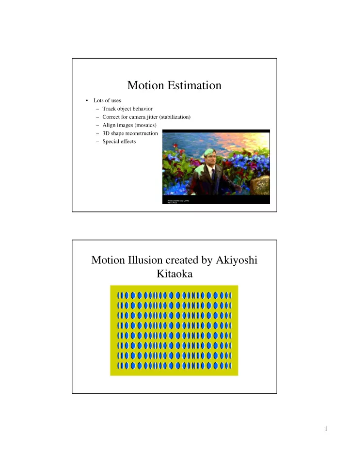
Motion Estimation

• Lots of uses

– Track object behavior – Correct for camera jitter (stabilization) – Align images (mosaics) – 3D shape reconstruction – Special effects

Motion Illusion created by Akiyoshi Kitaoka

2

Motion Illusion created by Akiyoshi Kitaoka

3

4

5

Optical flow

6

7

Aperture problem

8

Aperture problem

9

10

11

12

13

Hamburg Taxi Video

14

Hamburg Taxi Video Horn & Schunck Optical Flow

15

Fleet & Jepson Optical Flow

16

Tian & Shah Optical Flow Solving the Aperture Problem

• Basic idea: assume motion field is smooth
• Horn and Schunk: add smoothness term
• Lucas and Kanade: assume locally constant motion

– pretend the pixel’s neighbors have the same (u,v)

• If we use a 5x5 window, that gives us 25 equations per pixel!

– works better in practice than Horn and Schunk

17

Lucas-Kanade Flow

• How to get more equations for a pixel?

– Basic idea: impose additional constraints

• most common is to assume that the flow field is smooth locally
• one method: pretend the pixel’s neighbors have the same (u,v)

– If we use a 5x5 window, that gives us 25 equations per pixel!

– minimum least squares solution given by solution of:

Lucas-Kanade Flow

• Problem: more equations than unknowns

– The summations are over all pixels in the K x K window – This technique was first proposed by Lukas and Kanade (1981)

• Solution: solve least squares problem

18

Conditions for Solvability

– Optimal (u, v) satisfies Lucas-Kanade equation When is this solvable?

• ATA should be invertible
• ATA should not be too small due to noise

– eigenvalues λ1 and λ2 of ATA should not be too small

• ATA should be well-conditioned

– λ1/ λ2 should not be too large (λ1 = larger eigenvalue)

Eigenvectors of ATA

• Suppose (x,y) is on an edge. What is ATA?

– gradients along edge all point the same direction – gradients away from edge have small magnitude – is an eigenvector with eigenvalue – What’s the other eigenvector of ATA?

• let N be perpendicular to
• N is the second eigenvector with eigenvalue 0
• The eigenvectors of ATA relate to edge direction and magnitude

19

Edge

– large gradients, all the same

– large λ1, small λ2

Low Texture Region

– gradients have small magnitude

– small λ1, small λ2

20

High Texture Region

– gradients are different, large magnitudes

– large λ1, large λ2

Observation

• This is a two image problem BUT

– Can measure sensitivity by just looking at one of the images – This tells us which pixels are easy to track, which are hard

• very useful later on when we do feature tracking

21

Errors in Lucas-Kanade

• What are the potential causes of errors in this

procedure?

– Suppose ATA is easily invertible – Suppose there is not much noise in the image

• When our assumptions are violated

– Brightness constancy is not satisfied – The motion is not small – A point does not move like its neighbors

• window size is too large
• what is the ideal window size?

– Can solve using Newton’s method

• Also known as Newton-Raphson method

– Lucas-Kanade method does one iteration of Newton’s method

• Better results are obtained with more iterations

Improving Accuracy

• Recall our small motion assumption
• This is not exact

– To do better, we need to add higher order terms back in:

• This is a polynomial root finding problem

22

Iterative Refinement

• Iterative Lucas-Kanade Algorithm
• 1. Estimate velocity at each pixel by solving

Lucas-Kanade equations

• 2. Warp H towards I using the estimated flow field
• use image warping techniques
• 3. Repeat until convergence

Revisiting the Small Motion Assumption

• When is the motion small enough?

– Not if it’s much larger than one pixel (2nd order terms dominate) – How might we solve this problem?

23

Reduce the Resolution

image I image H

Gaussian pyramid of image H Gaussian pyramid of image I image I image H

u=10 pixels u=5 pixels u=2.5 pixels u=1.25 pixels

Coarse-to-Fine Optical Flow Estimation

24

image I image J

Gaussian pyramid of image H Gaussian pyramid of image I image I image H

Coarse-to-Fine Optical Flow Estimation

run iterative L-K run iterative L-K warp & upsample

. . .

Optical Flow Result

25

Spatiotemporal (x-y-t) Volumes

26

Visual Event Detection using Volumetric Features

• Y. Ke, R. Sukthankar, and M. Hebert, CMU,

CVPR 2005

• Goal: Detect motion events and classify actions

such as stand-up, sit-down, close-laptop, and grab-cup

• Use x-y-t features of optical flow

– Sum of u values in a cube – Difference of sum of v values in one cube and v values in an adjacent cube

27

3D Volumetric Features

Approximately 1 million features computed

Optical Flow Features

Optical flow of stand-up action (light means positive direction)

28

Classifier

• Cascade of binary classifiers that vote on the

classification of the volume

• Given a set of positive and negative examples at a

node, each feature and its optimal threshold is

• computed. Iteratively add filters at each node

until a target detection rate (e.g., 100%) or false positive rate (e.g., 20%) is achieved

• Output of the node is the majority vote of the

individual filters

Action Detection

• 78% - 92% detection rate on 4 action types: sit-

down, stand-up, close-laptop, grab-cup

• 0 – 0.6 false positives per minute
• Note: while lengths of actions vary, the first

frames are all aligned to a standard starting position for each action

• Classifier learns that beginning of video is more

discriminative than end because of variable length

• Relatively robust to viewpoint (< 45 degrees) and

scale (< 3x)

29

Results Structure-from-Motion

• Determining the 3-D structure of the world, and the motion
• f a camera (i.e., its extrinsic parameters) using a sequence
• f images taken by a moving camera

– Equivalently, we can think of the world as moving and the camera as fixed

• Like stereo, but the position of the camera isn’t known

(and it’s more natural to use many images with little motion between them, not just two with a lot of motion) and we have a long sequence of images, not just 2 images

– We may or may not assume we know the intrinsic parameters of the camera, e.g., its focal length

30

31

32

33

34

35

Results

• Look at paper figures…

Extensions

• Paraperspective

– [Poelman & Kanade, PAMI 97]

• Sequential Factorization

– [Morita & Kanade, PAMI 97]

• Factorization under perspective

– [Christy & Horaud, PAMI 96] – [Sturm & Triggs, ECCV 96]

• Factorization with Uncertainty

– [Anandan & Irani, IJCV 2002]

36

37 = [[e´]xF | e´]

38

39

• Sequential Structure and Motion

Computation

• !

" " # !

Sequential structure and motion recovery

• Initialize structure and motion from two views
• For each additional view

– Determine pose – Refine and extend structure

• Determine correspondences robustly by jointly

estimating matches and epipolar geometry

40

41

Pollefeys’ Result

42

Object Tracking

• 2D or 3D motion of known object(s)
• Recent survey: “Monocular model-based

3D tracking of rigid objects: A survey” available at http://www.nowpublishers.com/

43

44

45

46

47