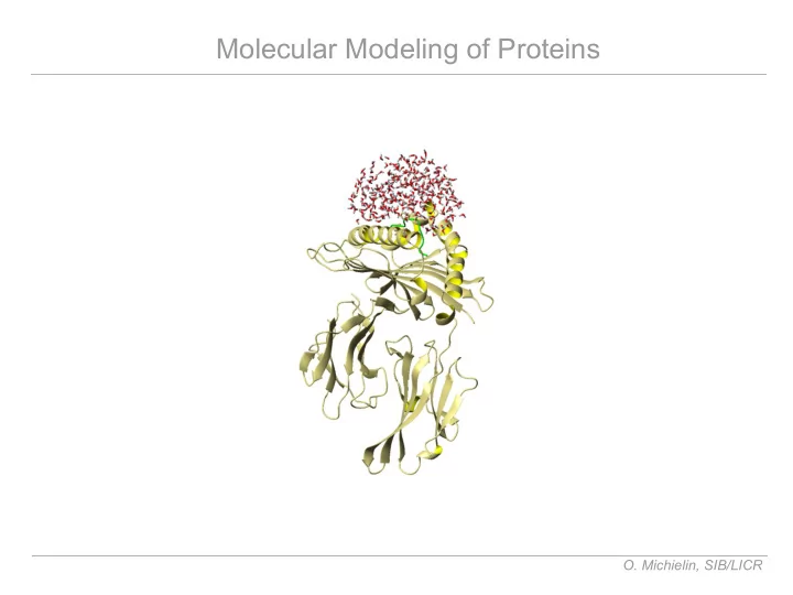
Molecular Modeling of Proteins O. Michielin, SIB/LICR Molecular - - PowerPoint PPT Presentation

• O. Michielin, SIB/LICR

Molecular Modeling of Proteins

• O. Michielin, SIB/LICR

Molecular Modeling of Proteins

Lecture Plan:

• Central role of partition function
• Review molecular interactions
• Modeling of molecular interactions: CHARMM force field
• Recent techniques:

implicit solvent models long range electrostatic treatment

• Molecular dynamics simulations
• elements of statistical mechanics
• microcanonical sampling
• canonical sampling
• isothermal-isobaric sampling
• Langevin dynamics
• Other sampling techniques
• Monte-Carlo
• Simulated Annealing (SA)
• Genetic Algorithms (GA)

• O. Michielin, SIB/LICR

Molecular Modeling: Introduction

What is Molecular Modeling? What is it good for?

Molecular Modeling is concerned with the description of the atomic and molecular interactions that govern microscopic and macroscopic behaviors of physical systems The essence of molecular modeling resides in the connection between the microscopic world and the macroscopic world provided by the theory of statistical mechanics Macroscopic

• bservable

(Solvation energy, affinity between two proteins, H-H distance, conformation, ... ) Average of observable

• ver selected microscopic

states

• O. Michielin, SIB/LICR

Connection micro/macroscopic: intuitive view

〈O〉= 1 Z ∑i Oie

− Ei

E1, P1 ~ e-bE1 E2, P2 ~ e-bE2 E3, P3 ~ e-bE3 E4, P4 ~ e-bE4 E5, P5 ~ e-bE5

Z=∑i e

− Ei

Where is the partition function Expectation value

• O. Michielin, SIB/LICR

Central Role of the Partition function

The determination of the macroscopic behavior of a system from a thermodynamical point of vue is tantamount to computing a quantity called the partition function, Z, from which all the properties can be derived.

Z=∑i e

− Ei

〈O〉= 1 Z ∑i Oie

− Ei

〈E〉= ∂ ∂ lnZ =U

p=kT  ∂lnZ  ∂V 

N ,T

A = -kT ln(Z)

. . .

Expectation Value Internal Energy Pressure Helmoltz free energy

• O. Michielin, SIB/LICR

Computation of the Partition function

The partition function is a very complex function to compute, and, in most cases, only numerical approximations are possible Numerical approximations require: 1) the computation of the energy of the system for microstate i

• performed using semi-empirical force fields

CHARMM / Amber / Gromos / ... 2) a method to sample all (or a representative portion) of the microstates accessible to the system in a given macroscopic state, i.e:

• microcanonical sampling for

fixed N,V,E systems

• canonical sampling for

fixed N,V,T systems

• isothermic-isobaric sampling for

fixed N,P,T systems

• ...

1) 2)

Z=∑i e

− Ei

• O. Michielin, SIB/LICR

Introduction & historical note

Theoretical milestones: Molecular dynamics milestones:

Newton (1643-1727): Classical equations of motion: F(t)=m a(t) Schrödinger (1887-1961): Quantum mechanical equations of motion:

• ih t (t)=H(t) (t)

Boltzmann(1844-1906): Foundations of statistical mechanics Metropolis (1953): First Monte Carlo (MC) simulation of a liquid (hard spheres) Wood (1957): First MC simulation with Lennard-Jones potential Alder (1957): First Molecular Dynamics (MD) simulation of a liquid (hard spheres) Rahman (1964): First MD simulation with Lennard-Jones potential Karplus (1977) & First MD simulation of proteins McCammon (1977) Karplus (1983): The CHARMM general purpose FF & MD program Kollman(1984): The AMBER general purpose FF & MD program Car-Parrinello(1985): First full QM simulations Kollmann(1986): First QM-MM simulations

Liquids Proteins

• O. Michielin, SIB/LICR

Molecular Interactions (I)

Bonded Interactions:

• Intramolecular energy terms associated with the deformation of the

electronic structure of the molecule. 3 terms are introduced in all FF: 1) Bond stretch 2) Angle bend 3) Dihedral torsion and a fourth one is often used to maintain planarity 4) Improper torsion

• O. Michielin, SIB/LICR

Molecular Interactions (II)

Non-Bonded Interactions:

• Inter and intramolecular energy terms arising from electrostatics

1) Electrostatic interactions Coulomb law: where e is the dielectric constant, 1 for vacuum, 4-20 for protein core, and 80 for water 2) van der Waals interactions Attractive part: due to induced-dipole/induced-dipole Repulsive part: due to Pauli exclusion principle Usually represented by the Lennard-Jones potential V Ele=∑

i j

qiq j 4 1 ri , j V vdW=∑

i j

4ij[ij/rij

12−ij/rij 6]

eij=(ei ej)1/2, sij = 1/2(si + sj) are obtained from the single atom param. e and s

• O. Michielin, SIB/LICR

Derived Interactions

Some interactions are often referred to as particular interactions, but they result from the two interactions previously described, i.e. the electrostatic and the van der Waals interactions. 1) Hydrogen bonds (Hb)

• Interaction of the type D-H ··· A
• The origin of this interaction is a

dipole-dipole attraction

• Typical ranges for distance and angle:

2.4 < d < 4.5Å and 180º < f < 90º 2) Hydrophobic effect

• Collective effect resulting from the energetically

unfavorable surface of contact between the water and an apolar medium (loss of water-water Hb)

• The apolar medium reorganizes to minimize the

water exposed surface

D H A f

• d

+d

d

Water Oil

• d

• O. Michielin, SIB/LICR

Semi-Empirical Force Fields

1) Goals of semi-empirical force fields

• Definition of empirical potential energy functions V(r) to model the

molecular interactions described previously

• These functions need to be differentiable in order to compute the

forces acting on each atom: F=-V(r)

2) Ways to compute semi-empirical potential energy functions

• First, theoretical analytical functional forms of the interactions are

derived

• The system is divided into a number of atom types that differ by their

atomic number and chemical environment, e.g. the carbons in C=O or C-C are not of the same type

• Parameters are determined so as to reproduce the interactions between

the various atom types by fitting procedures

• experimental enthalpies (CHARMM)
• experimental free energies (GROMOS, AMBER)

Parametrization available for proteins, lipids, sugars, ADN, ...

• O. Michielin, SIB/LICR

The CHARMM Force Field

 ∑

Impropers

K −0

2

 ∑

Dihedrals

K [1−cosn−]

∑

i j

4ij[ij/rij

12−ij/rij 6]

∑

i j

qi q j 4 1 ri , j V r=∑

Bonds

K bb−b0

2 ∑ Angles

K −0

2

• O. Michielin, SIB/LICR

The CHARMM 22 Parameter Set (Sample)

BONDS !V(bond) = Kb(b - b0)**2 !Kb: kcal/mole/A**2 !b0: A !atom type Kb b0 C C 600.000 1.3350 ! ALLOW ARO HEM ! Heme vinyl substituent (KK, from propene (JCS)) CA CA 305.000 1.3750 ! ALLOW ARO ! benzene, JES 8/25/89 CE1 CE1 440.000 1.3400 ! ! for butene; from propene, yin/adm jr., 12/95 CE1 CE2 500.000 1.3420 ! ! for propene, yin/adm jr., 12/95 ANGLES !V(angle) = Ktheta(Theta - Theta0)**2 !V(Urey-Bradley) = Kub(S - S0)**2 !Ktheta: kcal/mole/rad**2 !Theta0: degrees !Kub: kcal/mole/A**2 (Urey-Bradley) !S0: A !atom types Ktheta Theta0 Kub S0 CA CA CA 40.000 120.00 35.00 2.41620 ! ALLOW ARO ! JES 8/25/89 CE1 CE1 CT3 48.00 123.50 ! ! for 2-butene, yin/adm jr., 12/95 CE1 CT2 CT3 32.00 112.20 ! ! for 1-butene; from propene, yin/adm jr., 12/95 CE2 CE1 CT2 48.00 126.00 ! ! for 1-butene; from propene, yin/adm jr., 12/95 CE2 CE1 CT3 47.00 125.20 ! ! for propene, yin/adm jr., 12/95 DIHEDRALS !V(dihedral) = Kchi(1 - cos(n(chi) - delta)) !Kchi: kcal/mole !n: multiplicity !delta: degrees !atom types Kchi n delta C CT1 NH1 C 0.2000 1 180.00 ! ALLOW PEP ! ala dipeptide update for new C VDW Rmin, adm jr., 3/3/93c C CT2 NH1 C 0.2000 1 180.00 ! ALLOW PEP ! ala dipeptide update for new C VDW Rmin, adm jr., 3/3/93c C N CP1 C 0.8000 3 0.00 ! ALLOW PRO PEP ! 6-31g* AcProN CA CA CA CA 3.1000 2 180.00 ! ALLOW ARO ! JES 8/25/89 CA CPT CPT CA 3.1000 2 180.00 ! ALLOW ARO ! JWK 05/14/91 fit to indole IMPROPER !V(improper) = Kpsi(psi - psi0)**2 !Kpsi: kcal/mole/rad**2 !psi0: degrees !note that the second column of numbers (0) is ignored !atom types Kpsi psi0 CPB CPA NPH CPA 20.8000 0 0.0000 ! ALLOW HEM ! Heme (6-liganded): porphyrin macrocycle (KK 05/13/91) CPB X X C 90.0000 0 0.0000 ! ALLOW HEM ! Heme (6-liganded): substituents (KK 05/13/91) CT2 X X CPB 90.0000 0 0.0000 ! ALLOW HEM ! Heme (6-liganded): substituents (KK 05/13/91) CT3 X X CPB 90.0000 0 0.0000 ! ALLOW HEM ! Heme (6-liganded): substituents (KK 05/13/91) HA C C HA 20.0000 0 0.0000 ! ALLOW PEP POL ARO ! Heme vinyl substituent (KK, from propene (JCS)) HA CPA CPA CPM 29.4000 0 0.0000 ! ALLOW HEM

• O. Michielin, SIB/LICR

The CHARMM 22 Topology File (Tyr)

RESI TYR 0.00 GROUP ATOM N NH1 -0.47 ! | HD1 HE1 ATOM HN H 0.31 ! HN-N | | ATOM CA CT1 0.07 ! | HB1 CD1--CE1 ATOM HA HB 0.09 ! | | // \\ GROUP ! HA-CA--CB--CG CZ--OH ATOM CB CT2 -0.18 ! | | \ __ / \ ATOM HB1 HA 0.09 ! | HB2 CD2--CE2 HH ATOM HB2 HA 0.09 ! O=C | | GROUP ! | HD2 HE2 ATOM CG CA 0.00 GROUP ATOM CD1 CA -0.115 ATOM HD1 HP 0.115 GROUP ATOM CD2 CA -0.115 ATOM HD2 HP 0.115 GROUP ATOM CE1 CA -0.115 ATOM HE1 HP 0.115 GROUP ATOM CE2 CA -0.115 ATOM HE2 HP 0.115 GROUP ATOM CZ CA 0.11 ATOM OH OH1 -0.54 ATOM HH H 0.43 GROUP ATOM C C 0.51 ATOM O O -0.51 BOND CB CA CG CB CD2 CG CE1 CD1 BOND CZ CE2 OH CZ BOND N HN N CA C CA C +N BOND CA HA CB HB1 CB HB2 CD1 HD1 CD2 HD2 BOND CE1 HE1 CE2 HE2 OH HH DOUBLE O C CD1 CG CE1 CZ CE2 CD2 IMPR N -C CA HN C CA +N O DONOR HN N DONOR HH OH ACCEPTOR OH ACCEPTOR O C IC -C CA *N HN 1.3476 123.8100 180.0000 114.5400 0.9986 IC -C N CA C 1.3476 123.8100 180.0000 106.5200 1.5232 IC N CA C +N 1.4501 106.5200 180.0000 117.3300 1.3484 IC +N CA *C O 1.3484 117.3300 180.0000 120.6700 1.2287 IC CA C +N +CA 1.5232 117.3300 180.0000 124.3100 1.4513 IC N C *CA CB 1.4501 106.5200 122.2700 112.3400 1.5606 IC N C *CA HA 1.4501 106.5200 -116.0400 107.1500 1.0833 IC N CA CB CG 1.4501 111.4300 180.0000 112.9400 1.5113 IC CG CA *CB HB1 1.5113 112.9400 118.8900 109.1200 1.1119 IC CG CA *CB HB2 1.5113 112.9400 -123.3600 110.7000 1.1115 IC CA CB CG CD1 1.5606 112.9400 90.0000 120.4900 1.4064 IC CD1 CB *CG CD2 1.4064 120.4900 -176.4600 120.4600 1.4068 IC CB CG CD1 CE1 1.5113 120.4900 -175.4900 120.4000 1.4026 IC CE1 CG *CD1 HD1 1.4026 120.4000 178.9400 119.8000 1.0814 IC CB CG CD2 CE2 1.5113 120.4600 175.3200 120.5600 1.4022 IC CE2 CG *CD2 HD2 1.4022 120.5600 -177.5700 119.9800 1.0813 IC CG CD1 CE1 CZ 1.4064 120.4000 -0.1900 120.0900 1.3978 IC CZ CD1 *CE1 HE1 1.3978 120.0900 179.6400 120.5800 1.0799 IC CZ CD2 *CE2 HE2 1.3979 119.9200 -178.6900 119.7600 1.0798 IC CE1 CE2 *CZ OH 1.3978 120.0500 -178.9800 120.2500 1.4063 IC CE1 CZ OH HH 1.3978 119.6800 175.4500 107.4700 0.9594

• O. Michielin, SIB/LICR

Treatment of long range interactions

 ∑

i j ,rijvdW

4ij[ij/rij

12−ij/rij 6]

 ∑

i j ,rijEle

qi q j 4 1 ri , j

Introduction of dynamical cutoffs d Shift/ Switch

V r=∑

Bonds

k rr−r0

2 ∑ Angles

k −0

2

 ∑

Impropers

k −0

2  ∑ Dihedrals

k [1−cosn−]

• O. Michielin, SIB/LICR

Effect of cutoff values on energy calculations

8 Å cutoff No cutoff

Elec VdW Total Elec VdW Total

• O. Michielin, SIB/LICR

Major limitations of current force fields & perspectives

1) No electronic polarization:

• fixed partial charges allow

for conformational polarization but not electronic polarization

Problems Solutions

• Extended Lagrangian
• charges treated as dynamical

parameters

• QM-MM
• Full QM simulations
• Car-Parrinello

2) Quadratic form of potentials:

• problematic far from equilibrium

values

• no bond creation or deletion
• QM-MM
• Full QM simulations
• Car-Parrinello

• O. Michielin, SIB/LICR

Introduction to molecular surfaces

Solvent accessible Surface Connolly Surface Van der Waals Surface Rotating probe: radius 1.4 Å Definitions:

• Van der Waals: ensemble of van der Waals sphere centered at each atom
• Connolly:

ensemble of contact points between probe and vdW spheres

• Solvent:

ensemble of probe sphere centers

• O. Michielin, SIB/LICR

Examples of molecular surfaces

Van der Waals Solvent accessible Connolly (Contact)

• O. Michielin, SIB/LICR

e=1

Mapping properties on molecular surfaces

1) Electrostatic potential: surface elements are colored according to the value of f(x) with a linear scaling f(x) = -0.3 V  Red f(x) = 0.0 V  Gray f(x) = +0.3 V  Blue where f(x) is the solution of the Poisson-Boltzmann eq. 2) Other Properties: i) surface curvature ii) residue charge iii) residue conservation iv) ...

∇r∇ r=Macror∑

i

qi ni

0exp−qir

e=80

• O. Michielin, SIB/LICR

Implications of surface properties for ligand binding

Acetate (Negative charge) Toluene (Hydrophobic) Meguan (Positive charge)

• O. Michielin, SIB/LICR

Treatment of the solvent contribution

1) Explicit water molecule model: TIP3P, ... 2) Implicit solvent model:

• Based on Poisson-Boltzmann Equation:
• or an approximation...
• ACE potential

(Schaeffer & al.)

• SASA potential (Caflish & al.)
• EEF1 potential (Lazaridis & al.)

∇ r∇ r=Macror∑

i

qi ni

0exp−qir

e=80 e=1

O H H

• d

+d +d

For a discussion of theoretical aspects of implicit solvent models, see Roux & Simonson (Biophys. Chem. 1999, 78:1-20)

• O. Michielin, SIB/LICR

Minimal Input for Molecular Modeling

1) Topological properties: 2) Structural properties: 3) Energetical properties: description of the covalent connectivity of the molecules to be modeled the starting conformation of the molecule, provided by an X-ray structure, NMR data or a theoretical model a force field describing the force acting on each atom of the molecules 4) Thermodynamical properties: a thermodynamical ensemble that corresponds to the experimental conditions of the system, e.g. N,V,T , N,P,T, ...

T0 NV

• O. Michielin, SIB/LICR

Setup of a MD Simulation

• O. Michielin, SIB/LICR

Examples of MD Simulations

2) Vacuum Simulation of Melan-A Peptide 3) Explicit Solvent Simulation of Melan-A in p-MHC 1) Simulation of b2 microglobuline

• O. Michielin, SIB/LICR

Energy Landscape

Landscape for / plane of dialanine   Landscape for a protein

E 3N Spatial coordinates

• O. Michielin, SIB/LICR

Review of Statistical Mechanics

Thermodynamical Ensembles

Definition: a thermodynamical ensemble is a collection of microscopic states that all realize an identical macroscopic state A microscopic state of the system is given by a point (r, p) of the phase space of the system, where r= (r1, ..., rN ) and p= (p1, ..., pN ) are the positions and the momenta of the N atoms of the system. Examples of thermodynamical ensembles:

• Microcanonical:

fixed N, V, E

• ften used in MD
• Canonical:

fixed N, V, T

• ften used in MD
• Constant P-T:

fixed N, P, T

• ften used in MD
• Grand Canonic:

fixed m, P, T

• O. Michielin, SIB/LICR

Review of Statistical Mechanics

Boltzmann Distribution

Boltzmann showed that the canonical probability of the microstate i is given by

Pi= e

− Ei

∑

j

e

− E j= 1

Z e

− Ei

where Z is the partition function, b = 1/KBT with KB the Boltzmann constant. The partition function is a very complex function to compute, and in most cases only approximations can be obtained. All the properties of the system, micro or macroscopic, are contained in this function.

Illustration:

If a system can have two unique states, state (1) and state (2), then the ratio of systems in state (1) and (2) is

P1 P2 =e

− E1

e

− E2=e −E1−E2=e − E

at 300K, a DE of 1.3 kcal/mol results in a P1/P2 of 1 log10. (1) (2) Cave: if state (1) and (2) are composed of several microscopic states, DE  DG

• O. Michielin, SIB/LICR

Review of Statistical Mechanics

Expectation value

the macroscopic value of an observable, or expectation value, is given by the weighted average over all microscopic states of the thermodyna- mical Ensemble. In the case of a continuous microscopic ensemble,

〈O〉=

∫

Ens

O e

− E p ,rd p d r

∫

Ens

e

− E p ,rd p d r

=

∫

Ens

e

− K  pd p

∫

Ens

e

− K  pd p

∫

Ens

O e

−V rd r

∫

Ens

e

−V rd r

=

∫

Ens

O e

−V rd r

∫

Ens

e

−V rd r

= 1 Z ∫

Ens

O e

−V rd r

if O and V are not dependent upon p and E(p,r)=K(p)+V(r)

In the case of a discret set of microscopic states

〈O〉= 1 Z ∑

i

Oie

−V i

• O. Michielin, SIB/LICR

Ergodic Hypothesis

The ergodic hypothesis is that the ensemble averages used to compute expectation values can be replaced by time averages over the simulation. The microstates sampled by molecular dynamics are usually a small subset

• f the entire thermodynamical ensemble.

The validity of this hypothesis depends on the molecular modeling technique and on the quality of the sampling produced. The sampling should reach all important minima and explore them with the correct probability,

• NVE simulations

 Microcanonic ensemble  P = cst.

• NVT simulations

 Canonic ensemble  P(E) = e-bE

• NPT simulations

 Isothermic-isobaric ensemble  P(E) = e-b(E+PV) Note that the statistical weights are not present in the time average because of this fact.

〈O〉Ensemble = 1 Z∫O p ,qe

− E p ,qd pd q = 1

 ∫

t=0 

Otdt = 〈O〉Time

Ergodicity

• O. Michielin, SIB/LICR

 

E 3N Spatial coordinates

Ergodic Hypothesis: Intuitive view

NVE simulation in a local minimum

〈O〉Ensemble = 1 Z∫O,e

− E,d d  = 1

 ∫

t=0 

Otdt = 〈O〉Time

?

MD Trajectory

• O. Michielin, SIB/LICR

Lagrangian and Hamiltonian Formalism

Generalized coordinates

Lagrangian Hamiltonian

qi , ˙ qi

qi , pi= ∂ L ∂ ˙ qi

Equations of Motion d dt  ∂ L ∂ ˙ qi = ∂ L ∂qi

˙ qi=∂ H ∂ pi

Definition

Lqt, ˙ qt,t=K−V H qt, pt,t=∑i pi ˙ qi−Lqt, ˙ qt,t

˙ pi=−∂ H ∂qi Important properties

i=1,,3 N

∂ L ∂qi =0 ⇒ ∂ L ∂ ˙ qi

is a constant of motion if KK(t) and V=V(q,t) than H=K+V is the total energy if HH(t), the total energy is a constant of motion

i=1,,3 N

• O. Michielin, SIB/LICR

1) Microcanonical ensemble (constant N,V,E) sampling is obtained by finite difference method integrations of the dynamics equations:

• Verlet, Leap-Frog, Velocity Verlet, Gear

3) Isothermic-isobaric ensemble (constant N,P,T) sampling is obtained analogously to canonical sampling by 2 additional degrees of freedom and scaling of time ( T) and space ( P) 2) Canonical ensemble (constant N,V,T) sampling is obtained by two methods 1) Nose: additional degree of freedom s acting as an external system on the physical system. s introduces a scaling

• f time: dt = s dt.

2) Nose-Hoover: rewriting of the extended system equations to remove time scaling (which is hard to implement in MD) Integration of extended system by Verlet

MD Techniques (I): Sampling of the various ensembles MD Techniques (I): Sampling of the various ensembles

NVE T (Infinite Reservoir) NV T (Infinite Reservoir) N P (Infinite Reservoir)

• O. Michielin, SIB/LICR

MD Techniques (II): Microcanonical sampling

Several numerical methods have been developed to integrate these equations. One of the most stable integrator is that of Verlet: for a small time increment dt, one can use a Taylor expansion of the function r(t): mi ai=−∂ ∂ri r i=1, ..., N

ritt=ritvitt1/2aitt

2

rit−t=rit−vitt1/2aitt

2

Adding those equations, one gets r(t+dt) as a function of r(t) and r(t-dt).

ritt=2rit−rit−taitt

2

• In practice, this scheme is applied iteratively, starting from the initial conditions.
• Velocities are postcomputed as v(t) = [r(t+dt)-r(t-dt)] / 2dt.
• Positions are correct up to dt4 and velocities to dt2.
• This scheme conserves energy with very good accuracy.

For an Hamiltonian of the form in cartesian coordinates, the Hamilton equations of motion reduce to the Newton equations

H  p ,r=∑

i=1 3 N

pi

2

2mi r1 ,,r3 N

˙ ri= pi mi

• O. Michielin, SIB/LICR

MD Techniques (III): Canonical sampling

The system is here coupled to an external infinite constant temperature bath. The coupling to the physical system is done by an additional degree of freedom s and a scaling of the time such that dt' = dt / s. Therefore qi'=qi and pi'=pi/s, where (qi',pi',t') are the real variables and (qi,pi,t) the virtual variables. The Hamiltonian for the extended system is H  p ,q , ps , s=∑

i N

pi

2

2mi s

2q ps 2

2Q 3 N 1kT ln s and the equations of motion are

˙ qi=∂ H ∂ pi = pi mi s

2

˙ pi=−∂ H ∂qi =−∂ ∂qi

(Equations for p and q)

˙ s=∂ H ∂ ps = ps Q ˙ ps=−∂ H ∂ s =1 s∑

i=1 N

[ pi

2

mi s

2−3 N −1kT ]

(Equations for ps and s)

See Nose 1984, J. Chem. Phys. 81(1): 511-19

• O. Michielin, SIB/LICR

MD Techniques (IV): Derivation of canonical ensemble for HNose

The microcanonical partition function associated to the Nose extended Hamiltonian is of the form Z=∫dps∫ds∫ d p∫ d q [H 0 p/s ,q ps

2/2Q3 N 1kT ln s−E]

where is the unextended physical Hamiltonian. The volume element dpdq = s3N dp'dq', therefore

H 0 p ,q=∑

i=1 N

pi

2

2mi q

Z=∫dps∫d p'∫d q'∫ds s

3 N [H 0 p' ,q' ps 2/2Q3 N 1kT ln s−E]

and using d[f(s)] = d(s-s0) / f'(s0) with s0 the root of f(s), on gets Z=C∫d p'∫d q' exp[−H 0 p' ,q' /kT ] which is the partition function of the physical system in the canonical ensemble except for a constant factor

• O. Michielin, SIB/LICR

H =∑

i N

pi

2

2mi s

2V 2/3V 1/3q ps 2

2Q 3 N 1kT ln s pV

2

2W PexV

MD Techniques (V): Isothermic-Isobaric sampling

The system is here coupled to an external infinite thermostat and to a barostat. The coupling to the physical system is done by two additional degrees of freedom s and V. Analogously, a scaling of time and of the spatial coordinates is performed. The virtual variables (qi,pi,s,V,t) are related to the real variables (qi',pi',s,V,t') by the relations dt' = dt / s, qi'= V1/3qi and pi'= pi / V1/3s. The Hamiltonian for the extended system is

T (Infinite Reservoir) P (Infinite Reservoir)

s V

• O. Michielin, SIB/LICR

MD Techniques (VI): NTP ensemble equations of motion

˙ qi=∂ H ∂ pi = pi miV

2/3 s 2

˙ s=∂ H ∂ ps = ps Q ˙ pi=−∂ H ∂qi =−∂ ∂qi =−∂ ∂qi' V

1/3

˙ ps=−∂ H ∂ s =1 s ∑

i=1 N

[ pi

2

miV

2/3 s 2−3 N −1kT ]

H =∑

i N

pi

2

2mi s

2V 2/3V 1/3q ps 2

2Q 3 N 1kT ln s pV

2

2W PexV Using the extended Hamiltonian with thermostat and barostat coupling the following equations of motion are derived (Equations for p and q) (Equations for ps and s)

dV dt = ∂ H ∂ pV = pV W (Equations for pV and V)

˙ pV=−∂ H ∂V = 1 3V −Pex [∑

i=1 N

 pi

2

miV

2/3 s 2− ∂

∂qi' qi']

• O. Michielin, SIB/LICR

MD Techniques (VII): Derivation of NTP ensemble for HNose

The microcanonical partition function associated to the Nose extended NTP Hamiltonian is of the form Z=∫dpV∫dV∫dps∫ds∫d p∫d q [H 0 p/sV

1/3 ,V 1/3q ps 2

2Q  pv

2

2W PexV 3 N 1kT ln s−E] where again is the unextended physical Hamiltonian. Similarly to the case of the canonical ensemble, on can show that Z=C∫d p'∫ d q' exp[−H 0 p' ,q'PexV /kT ] which is the partition function of the physical system in the NTP ensemble except for a constant factor

H 0 p ,q=∑

i=1 N

pi

2

2mi q

• O. Michielin, SIB/LICR

Other sampling methods: I

Langevin Dynamics (LD)

In Langevin Dynamics, two additional forces are added to the standard force field:

• a friction force:
• gi pi

whose direction is opposed to the velocity of atom i

• a stochastic (random) force:

z(t) such that <z (t)> = 0. This leads to the following equation for the motion of atom i: This equation can for example simulate the friction and stochastic effect of the solvent in implicit solvent simulations. The temperature is adjusted via g and z, using the dissipation-fluctuation theorem. The stochastic term can improve barrier crossing and hence sampling.

Cave: LD does not produce a canonical ensemble

˙ qi= pi m , ˙ pi=F iq ,−i pit

• O. Michielin, SIB/LICR

Other sampling methods: II

Monte Carlo Simulations and the Metropolis criterion

In this sampling method, instead of computing the forces on each atom to solve its time evolution, random movements are assigned to the system and the potential energy of the resulting conformer is evaluated. To insure Boltzmann sampling, additional criteria need to be applied on the new conformer. Let C be the initial conformer and C' the randomly modified:

• if V(C') < V(C), the new conformer is kept and C' becomes C for next step
• if V(C') > V(C), a random number, r, in the [0,1] interval is generated and

if e-b(V'-V) > r, the new conformer is kept and C' becomes C for next step Using this algorithm, one insures Boltzmann statistics, PC '  PC =e

−V '−V 

• O. Michielin, SIB/LICR

Other sampling methods: III

Simulated annealing (SA) and simulated quenching (SQ)

?

In these techniques, the temperature of the system is raised and cooled several times during a standard MD, LD or MC simulation. Two different types of cooling can be achived:

• a slow (logarithmic) protocol: annealing
• a fast (exponential) protocol: quenching

This allows to pass over free energy barriers and to find other minima. The sampling obtained by SA generates of an ensemble that tends to a Boltzmann distribution as the cooling time tends to infinity. The sampling obtained by SQ does not follow a Boltzmann distribution.

• O. Michielin, SIB/LICR

Conclusion

Molecular dynamics and other sampling techniques allow:

Sampling of the conformational space of the molecule according to various thermodynamical systems:

• following an isoenergetic surface (microcanonic)
• following an isothermic and/or isobaric surface (canonic, constant TP)
• probability of state is related

to its free energy

• macroscopic quantities can be
• btained as averages over the trajectory, the ergodic hypothesis

〈O〉Ensemble=〈O〉Time= 1  ∫

t=0 

Otdt

• O. Michielin, SIB/LICR

Some Applications of Molecular Dynamics Techniques

1) Equilibrium MD simulations

• Expectation values (macroscopic observables)
• using ergodic hypothesis
• Fluctuations
• correlation RMSD/B-Factors
• Free energies
• absolute values

3) Non-Equilibrium MD simulations

• Study of large conformational changes
• Domain dynamics
• Docking
• Protein Folding / Stucture predictions

2) Quasi-Equilibrium MD simulations

• Free energy differences between closely related molecules
• conformational free energy change
• alchemical mutations

• O. Michielin, SIB/LICR

References

1) Online

• http://cmm.info.nih.gov/intro_simulation/course_for_html.html
• http://www.ch.embnet.org/MD_tutorial
• http://www.biophysics.org/btol/img/Beard.D.pdf

2) Textbooks

Statistical Mechanics

• D. A. McQuarrie: Statistical Mechanics
• R. K. Pathria: Statistical Mechanics
• D. Chandler: Introduction to Modern Statistical Mechanics
• R. P. Feynman: Statistical Mechanics. A Set of Lectures

Molecular Dynamics

• Allen & Tildesley: Computer Simulations of Liquids
• Tidor & Karplus: Proteins

Electrodynamics

• J. D. Jackson: Classical Electrodynamics

Protein Structure

• T. E. Creighton: Proteins. Structures and molecular properties