DNA Binding Proteins CSE 527 Autumn 2007 A variety of DNA binding - - PowerPoint PPT Presentation

dna binding proteins cse 527
SMART_READER_LITE
LIVE PREVIEW

DNA Binding Proteins CSE 527 Autumn 2007 A variety of DNA binding - - PowerPoint PPT Presentation

DNA Binding Proteins CSE 527 Autumn 2007 A variety of DNA binding proteins (transcription factors; a significant fraction, Lectures 8-9 (& part of 10) perhaps 5-10%, of all human proteins) Motifs: Representation & Discovery


slide-1
SLIDE 1

1

CSE 527

Autumn 2007

Lectures 8-9 (& part of 10) Motifs: Representation & Discovery

2

DNA Binding Proteins

A variety of DNA binding proteins (“transcription factors”; a significant fraction, perhaps 5-10%, of all human proteins) modulate transcription of protein coding genes

3

The Double Helix

Los Alamos Science 4
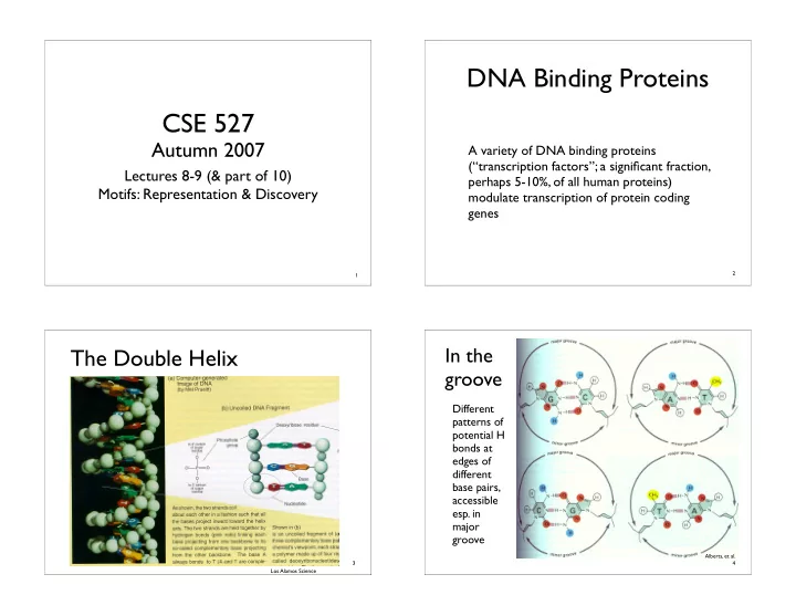
In the groove

Different patterns of potential H bonds at edges of different base pairs, accessible

  • esp. in

major groove

Alberts, et al.

slide-2
SLIDE 2

5 Alberts, et al.

Helix-Turn-Helix DNA Binding Motif

6

H-T

  • H Dimers

Bind 2 DNA patches, ~ 1 turn apart Increases both specificity and affinity

Alberts, et al. 7

Zinc Finger Motif

Alberts, et al. 8

Leucine Zipper Motif

Homo-/hetero-dimers and combinatorial control

Alberts, et al.

slide-3
SLIDE 3

9

Some Protein/DNA interactions well-understood

10

But the overall DNA binding “code” still defies prediction

11

Bacterial Met Repressor

SAM (Met derivative)

Alberts, et al.

a beta-sheet DNA binding domain

Negative feedback loop: high Met level ⇒ repress Met synthesis genes

12

DNA binding site summary

  • complex “code”
  • short patches (6-8 bp)
  • often near each other (1 turn = 10 bp)
  • often reverse-complements
  • not perfect matches
slide-4
SLIDE 4

13

Sequence Motifs

Last few slides described structural motifs in proteins Equally interesting are the DNA sequence motifs to which these proteins bind - e.g. ,

  • ne leucine zipper dimer might bind (with

varying affinities) to dozens or hundreds of similar sequences

14

  • E. coli Promoters

“TATA Box” ~ 10bp upstream of transcription start How to define it? Consensus is TATAAT BUT all differ from it Allow k mismatches? Equally weighted? Wildcards like R,Y? ({A,G}, {C,T}, resp.)

TACGAT TAAAAT TATACT GATAAT TATGAT TATGTT

15

  • E. coli Promoters
  • “TATA Box” - consensus TATAAT ~

10bp upstream of transcription start

  • Not exact: of 168 studied (mid 80’s)

– nearly all had 2/3 of TAxyzT – 80-90% had all 3 – 50% agreed in each of x,y,z – no perfect match

  • Other common features at -35, etc.

16

TATA Box Frequencies

pos base

1 2 3 4 5 6 A 2 95 26 59 51 1 C 9 2 14 13 20 3 G 10 1 16 15 13 T 79 3 44 13 17 96

slide-5
SLIDE 5

17

TATA Scores

pos base

1 2 3 4 5 6 A

  • 36

19 1 12 10

  • 46

C

  • 15
  • 36
  • 8
  • 9
  • 3
  • 31

G

  • 13
  • 46
  • 6
  • 7
  • 9 -46(?)

T 17

  • 31

8

  • 9
  • 6

19

18

Scanning for TATA

Stormo, Ann. Rev. Biophys. Biophys Chem, 17, 1988, 241-263

A C G T A C G T A C G T

19

Score Distribution

(Simulated)

500 1000 1500 2000 2500 3000 3500

  • 150
  • 130
  • 110
  • 90
  • 70
  • 50
  • 30
  • 10

10 30 50 70 90

20

Weight Matrices: Statistics

Assume: fb,i = frequency of base b in position i in TATA fb = frequency of base b in all sequences Log likelihood ratio, given S = B1B2...B6:

  • =
= =
  • =
  • =
  • 6
1 , 6 1 6 1 , log log er”) “nonpromot | P(S ) “promoter” | P(S log i B i B i B i i B i i i i f f f f

Assumes independence

slide-6
SLIDE 6

21

Neyman-Pearson

Given a sample x1, x2, ..., xn, from a distribution f (...|) with parameter , want to test hypothesis = 1 vs = 2. Might as well look at likelihood ratio: f(x1, x2, ..., xn|1) f(x1, x2, ..., xn|2)

(or log likelihood ratio)

>

22

Score Distribution (Simulated)

500 1000 1500 2000 2500 3000 3500

  • 150
  • 130
  • 110
  • 90
  • 70
  • 50
  • 30
  • 10

10 30 50 70 90

23

What’s best WMM?

Given 20 sequences s1, s2, ..., sk of length 8, assumed to be generated at random according to a WMM defined by 8 x (4-1) parameters , what’s the best ? E.g., what’s MLE for given data s1, s2, ..., sk? Answer: count frequencies per position.

24

Weight Matrices: Chemistry

Experiments show ~80% correlation of log likelihood weight matrix scores to measured binding energy of RNA polymerase to variations on TATAAT consensus [Stormo & Fields]

slide-7
SLIDE 7

25

ATG ATG ATG ATG ATG GTG GTG TTG Freq. Col 1 Col 2 Col3 A .625 C G .250 1 T .125 1 LLR Col 1 Col 2 Col 3 A 1.32

  • C
  • G
  • 2.00

T

  • 1.00

2.00

  • Another WMM example

log2 fxi,i fxi , fxi = 1 4

8 Sequences: Log-Likelihood Ratio:

26

  • E. coli - DNA approximately 25% A, C, G, T
  • M. jannaschi - 68% A-T, 32% G-C

LLR from previous example, assuming e.g., G in col 3 is 8 x more likely via WMM than background, so (log2) score = 3 (bits).

LLR Col 1 Col 2 Col 3 A .74

  • C
  • G

1.00

  • 3.00

T

  • 1.58

1.42

  • Non-uniform Background

fA = fT = 3/8 fC = fG = 1/8

27

AKA Kullback-Liebler Distance/Divergence, AKA Information Content Given distributions P , Q

Notes:

Relative Entropy

H(P||Q) =

  • x∈Ω

P(x) log P(x) Q(x)

Undefined if 0 = Q(x) < P(x) Let P(x) log P(x) Q(x) = 0 if P(x) = 0 [since lim

y→0 y log y = 0]

28

WMM: How “Informative”? Mean score of site vs bkg?

For any fixed length sequence x, let P(x) = Prob. of x according to WMM Q(x) = Prob. of x according to background Relative Entropy: H(P||Q) is expected log likelihood score of a sequence randomly chosen from WMM;

  • H(Q||P) is expected score of Background

H(P||Q) =

  • x∈Ω

P(x) log2 P(x) Q(x)

H(P||Q)

  • H(Q||P)
slide-8
SLIDE 8

29

WMM Scores vs Relative Entropy

500 1000 1500 2000 2500 3000 3500

  • 150
  • 130
  • 110
  • 90
  • 70
  • 50
  • 30
  • 10

10 30 50 70 90

  • H(Q||P) = -6.8

H(P||Q) = 5.0 For WMM, you can show (based on the assumption of independence between columns), that : where Pi and Qi are the WMM/background distributions for column i.

H(P||Q) =

  • i H(Pi||Qi)

31

Freq. Col 1 Col 2 Col3 A .625 C G .250 1 T .125 1 LLR Col 1 Col 2 Col 3 A 1.32

  • C
  • G
  • 2.00

T

  • 1.00

2.00

  • RelEnt

.70 2.00 2.00 4.70 LLR Col 1 Col 2 Col 3 A .74

  • C
  • G

1.00

  • 3.00

T

  • 1.58

1.42

  • RelEnt

.51 1.42 3.00 4.93

WMM Example, cont.

Uniform Non-uniform

32

Pseudocounts

Are the -’s a problem? Certain that a given residue never occurs in a given position? Then - just right Else, it may be a small-sample artifact Typical fix: add a pseudocount to each observed count—small constant (e.g., .5, 1) Sounds ad hoc; there is a Bayesian justification

slide-9
SLIDE 9

33

WMM Summary

  • Weight Matrix Model (aka Position Specific Scoring Matrix,

PSSM, “possum”, 0th order Markov models)

  • Simple statistical model assuming independence

between adjacent positions

  • To build: count (+ pseudocount) letter frequency per

position, log likelihood ratio to background

  • To scan: add LLRs per position, compare to threshold
  • Generalizations to higher order models (i.e., letter

frequency per position, conditional on neighbor) also possible, with enough training data

34

How-to Questions

Given aligned motif instances, build model?

  • Frequency counts (above, maybe with pseudocounts)

Given a model, find (probable) instances

  • Scanning, as above

Given unaligned strings thought to contain a motif, find it? (e.g., upstream regions for co-expressed

genes from a microarray experiment)

  • Hard... rest of lecture.

35

Motif Discovery

Unfortunately, finding a site of max relative entropy in a set of unaligned sequences is NP-hard [Akutsu]

36

Motif Discovery: 4 example approaches

Brute Force Greedy search Expectation Maximization Gibbs sampler

slide-10
SLIDE 10

37

Brute Force

Input:

  • Seqs s1, s2, ..., sk (len ~n, say), each w/ one instance
  • f an unknown length l motif

Algorithm:

  • create singleton set with each length l

subsequence of each s1, s2, ..., sk (~nk sets)

  • for each set, add each possible length l

subsequence not already present (~n2k(k-1) sets)

  • repeat until all have k sequences (~nkk! sets)
  • compute relative entropy of each; pick best

problem: astronomically sloooow

38

Greedy Best-First Approach

[Hertz & Stormo]

Input:

  • Sequence s1, s2, ..., sk; motif length I; “breadth” d

Algorithm:

  • create singleton set with each length l

subsequence of each s1, s2, ..., sk

  • for each set, add each possible length l

subsequence not already present

  • compute relative entropy of each
  • discard all but d best
  • repeat until all have k sequences

usual “greedy” problems

X X X

39

Yi,j = 1 if motif in sequence i begins at position j

  • therwise

Expectation Maximization

[MEME, Bailey & Elkan, 1995]

Input (as above): Sequence s1, s2, ..., sk; motif length l; background model; again assume one instance per sequence (variants possible) Algorithm: EM Visible data: the sequences Hidden data: where’s the motif Parameters : The WMM

40

MEME Outline

Typical EM algorithm:

  • Parameters t at tth iteration, used to estimate

where the motif instances are (the hidden variables)

  • Use those estimates to re-estimate the parameters

to maximize likelihood of observed data, giving t+1

  • Repeat

Key: given a few good matches to best motif, expect to pick out more

slide-11
SLIDE 11

41

  • Yi,j

= E(Yi,j | si, θt) = P(Yi,j = 1 | si, θt) = P(si | Yi,j = 1, θt) P (Yi,j=1|θt)

P (si|θt)

= cP(si | Yi,j = 1, θt) = c l

k=1 P(si,j+k−1 | θt)

where c is chosen so that

j

Yi,j = 1.

E = 0 · P(0) + 1 · P(1) Bayes

Expectation Step

(where are the motif instances?)

1 3 5 7 9 11 ...

Sequence i

  • Yi,j }

=1

42

Q(θ | θt) = EY ∼θt[log P(s, Y | θ)] = EY ∼θt[log k

i=1 P(si, Yi | θ)]

= EY ∼θt[k

i=1 log P(si, Yi | θ)]

= EY ∼θt[k

i=1

|si|−l+1

j=1

Yi,j log P(si, Yi,j = 1 | θ)] = EY ∼θt[k

i=1

|si|−l+1

j=1

Yi,j log(P(si | Yi,j = 1, θ)P(Yi,j = 1 | θ))] = k

i=1

|si|−l+1

j=1

EY ∼θt[Yi,j] log P(si | Yi,j = 1, θ) + C = k

i=1

|si|−l+1

j=1

  • Yi,j log P(si | Yi,j = 1, θ) + C

Maximization Step

(what is the motif?)

Find maximizing expected value: Exercise: Show this is maximized by “counting” letter frequencies over all possible motif instances, with counts weighted by , again the “obvious” thing.

M-Step (cont.)

Q(θ | θt) = k

i=1

|si|−l+1

j=1

  • Yi,j log P(si | Yi,j = 1, θ) + C
  • Yi,j

s1 :

  • ACGGATT. . .

. . . sk :

  • GC. . . TCGGAC
  • Y1,1

ACGG

  • Y1,2

CGGA

  • Y1,3

GGAT . . . . . .

  • Yk,l−1

CGGA

  • Yk,l

GGAC

44

Initialization

  • 1. Try every motif-length substring, and use as

initial a WMM with, say 80% of weight on that sequence, rest uniform

  • 2. Run a few iterations of each
  • 3. Run best few to convergence

(Having a supercomputer helps)

slide-12
SLIDE 12

The Gibbs Sampler

Lawrence, et al. “Detecting Subtle Sequence Signals: A Gibbs Sampling Strategy for Multiple Sequence Alignment,” Science 1993

Another Motif Discovery Approach

Geman & Geman, IEEE PAMI 1984 Hastings, Biometrika, 1970 Metropolis, Rosenbluth, Rosenbluth, Teller, & Teller, “Equations of State Calculations by Fast Computing Machines,” J. Chem. Phys. 1953 Josiah Williard Gibbs, 1839-1903, American physicist, a pioneer of thermodynamics

Some History

slide-13
SLIDE 13

How to Average

An old problem: n random variables: Joint distribution (p.d.f.): Some function: Want Expected Value:

x1, x2, . . . , xk P(x1, x2, . . . , xk) E(f(x1, x2, . . . , xk)) f(x1, x2, . . . , xk)

How to Average

Approach 1: direct integration (rarely solvable analytically, esp. in high dim) Approach 2: numerical integration (often difficult, e.g., unstable, esp. in high dim) Approach 3: Monte Carlo integration sample and average:

E(f(x1, x2, . . . , xk)) =

  • x1
  • x2

· · ·

  • xk

f(x1, x2, . . . , xk) · P(x1, x2, . . . , xk)dx1dx2 . . . dxk

E(f( x)) ≈ 1

n

n

i=1 f(

x(i))

  • x(1),

x(2), . . . x(n) ∼ P( x)

Markov Chain Monte Carlo (MCMC)

  • Independent sampling also often hard, but not

required for expectation

  • MCMC w/ stationary dist = P
  • Simplest & most common: Gibbs Sampling
  • Algorithm

for t = 1 to for i = 1 to k do :

P(xi | x1, x2, . . . , xi−1, xi+1, . . . , xk)

xt+1,i ∼ P(xt+1,i | xt+1,1, xt+1,2, . . . , xt+1,i−1, xt,i+1, . . . , xt,k)

t+1 t

  • Xt+1 ∼ P(

Xt+1 | Xt)

1 3 5 7 9 11 ... Sequence i

  • Yi,j
slide-14
SLIDE 14
  • Input: again assume sequences s1, s2, ..., sk

with one length w motif per sequence

  • Motif model: WMM
  • Parameters: Where are the motifs?

for 1 i k, have 1 xi |si|-w+1

  • “Full conditional”: to calc

build WMM from motifs in all sequences except i, then calc prob that motif in ith seq

  • ccurs at j by usual “scanning” alg.

P(xi = j | x1, x2, . . . , xi−1, xi+1, . . . , xk)

54

Randomly initialize xi’s for t = 1 to for i = 1 to k discard motif instance from si; recalc WMM from rest for j = 1 ... |si|-w+1 calculate prob that ith motif is at j: pick new xi according to that distribution

Similar to MEME, but it would average over, rather than sample from

P(xi = j | x1, x2, . . . , xi−1, xi+1, . . . , xk)

Overall Gibbs Alg

Burnin - how long must we run the chain to reach stationarity? Mixing - how long a post-burnin sample must we take to get a good sample of the stationary distribution? (Recall that individual samples are not independent, and may not “move” freely through the sample space. Also, many isolated modes.)

Issues

“Phase Shift” - may settle on suboptimal solution that overlaps part of motif. Periodically try moving all motif instances a few spaces left or right. Algorithmic adjustment of pattern width: Periodically add/remove flanking positions to maximize (roughly) average relative entropy per position Multiple patterns per string

Variants & Extensions

slide-15
SLIDE 15

60

  • 13 tools
  • Real ‘motifs’ (Transfac)
  • 56 data sets (human, mouse, fly, yeast)
  • ‘Real’, ‘generic’, ‘Markov’
  • Expert users, top prediction only

Methodology

slide-16
SLIDE 16

* * $ * ^ ^ ^ * *

$ Greed * Gibbs ^ EM

63

Lessons

  • Evaluation is hard (esp. when “truth” is unknown)
  • Accuracy low
  • partly reflects defects in evaluation methodology

(e.g. <= 1 prediction per data set; results better in synth data)

  • partly reflects difficult task, limited knowledge

(e.g. yeast > others)

  • No clear winner re methods or models

64

Motif Discovery Summary

  • Important problem: a key to understanding gene

regulation

  • Hard problem: short, degenerate signals amidst much

noise

  • Many variants have been tried, for representation,

search, and discovery. We looked at only a few:

  • Weight matrix models for representation & search
  • greedy, MEME and Gibbs for discovery
  • Still much room for improvement. Comparative

genomics, i.e. cross-species comparison is very promising