ARX Model Development IIT Bombay Consider data obtained from two - - PowerPoint PPT Presentation

Automation Lab IIT Bombay

System Identification 69 4/10/2012 System Identification 69

ARX Model Development

) ( ) 3 ( ) 2 ( ) 2 ( ) 1 ( ) ( ˆ .......... ) 4 ( ) 1 ( ) 2 ( ) 2 ( ) 3 ( ) 4 ( ˆ

2 1 2 1 2 1 2 1

N e N u b N u b N y a N y a N y e u b u b y a y a y + − + − + − − − − = + + + − − =

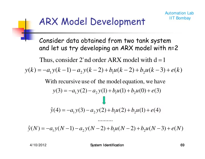
) ( ) 3 ( ) 2 ( ) 2 ( ) 1 ( ) ( 1 d with model ARX

• rder

nd 2' consider Thus,

2 1 2 1

k e k u b k u b k y a k y a k y + − + − + − − − − = =

Consider data obtained from two tank system and let us try developing an ARX model with n=2

) 3 ( ) ( ) 1 ( ) 1 ( ) 2 ( ) 3 ( have we equation, model the

• f

use recursive With

2 1 2 1

e u b u b y a y a y + + + − − =

Automation Lab IIT Bombay

System Identification 70 4/10/2012 System Identification 70

ARX : Parameter Identification

{

4 3 4 2 1 4 4 4 4 4 4 4 4 4 3 4 4 4 4 4 4 4 4 4 2 1 4 3 4 2 1 e θ Y ⎥ ⎥ ⎥ ⎥ ⎦ ⎤ ⎢ ⎢ ⎢ ⎢ ⎣ ⎡ + ⎥ ⎥ ⎥ ⎥ ⎦ ⎤ ⎢ ⎢ ⎢ ⎢ ⎣ ⎡ Ω ⎥ ⎥ ⎥ ⎥ ⎦ ⎤ ⎢ ⎢ ⎢ ⎢ ⎣ ⎡ − − − − − − − − − − = ⎥ ⎥ ⎥ ⎥ ⎦ ⎤ ⎢ ⎢ ⎢ ⎢ ⎣ ⎡ e(N) ... ) e( ) e( b b a a N u N u N y N y u u y y u u y y y(N) ... ) y( ) y( 4 3 ) 3 ( ) 2 ( ) 2 ( ) 1 ( .. .. .. .. ) 1 ( ) 2 ( ) 2 ( ) 3 ( ) ( ) 1 ( ) 1 ( ) 2 ( 4 3

2 1 2 1

form matrix in Arranging

“Linear in Parameter” Model Advantage: Least square parameter estimation problem can be solved analytically

e θ Y + Ω =

Automation Lab IIT Bombay

System Identification 71 4/10/2012 System Identification 71

ARX : Parameter Identification

[ ] [ ]

θ θ Y θ Y e e = ⎥ ⎦ ⎤ ⎢ ⎣ ⎡ ∂ ∂ ∂ ∂ ∂ ∂ ∂ ∂ = ∂ ∂ Ω − Ω − = =

T T T

b b a a

2 1 2 1

• ptimality

for condition Necessary : Function Objective ϕ ϕ ϕ ϕ ϕ ϕ

[ ]

e e θ θ

T

min ) ( ) , , , ( min ˆ estimation parameter square Least

2 2 2 1 2 1

= =

∑

= N k

k e b b a a

[ ] [ ] [ ]

θ Y θ θ Y θ Y θ = Ω − Ω − = ∂ Ω − Ω − ∂ = ∂ ∂

T T

ϕ

Automation Lab IIT Bombay

System Identification 72 4/10/2012 System Identification 72

ARX : Parameter Identification

[ ]

Y θ

T T LS

Ω Ω Ω = ⇒

−1

ˆ

definite positive is matrix Hessian minimum be to

• ptimum

for condition ufficient

2 2

⎥ ⎦ ⎤ ⎢ ⎣ ⎡ ∂ ∂ θ ϕ S

ϕ ϕ

• f

minimum global be to happens it fact, In minimum a is ˆ definite ve always is which

2 2 LS T

θ θ ⇒ + Ω Ω = ⎥ ⎦ ⎤ ⎢ ⎣ ⎡ ∂ ∂

q 0.01191 q 0.002506 B(q) q 0.5876 q 1.558

• 1

) A(q e(k) )u(k) B(q )y(k) A(q

3

• 2
• 2
• 1
• 1
• 1
• 1

+ = + = + =

Least square Estimates for Two tank system

Automation Lab IIT Bombay

System Identification 73

ARX Model: Output and Residuals

50 100 150 200 250

• 1
• 0.5

0.5 1 y(k)

ARX Model ARX(2,2,2): Comparison of Predicted and Measured Outputs

50 100 150 200 250

• 0.1
• 0.05

0.05 0.1 e(k) Time (samples)

Automation Lab IIT Bombay

System Identification 74

Model Residuals

4/10/2012 System Identification 74

{e(k)}

• f

Function ation Autocorrel Check sequence? noise white a form ˆ ˆ ˆ model ARX

• rder

ns 2'

• f

residues the model Do : Question Y Y θ Y e − = Ω − =

LS

Model fit appears to be much better than OE

• model. But, this can be deceptive. How do we

assess the model quality? Checks

{e(k)}. and {u(k)} between n correlatio cross Check {e(k)}? residuals in left still 'signal'

• f

part some Is : Question

Automation Lab IIT Bombay

System Identification 75

ARX(2,2,2): Correlation Functions

5 10 15 20 25

• 0.5

0.5 1 1.5 ARX Model ARX(2,2,2): Correlation function of residuals e(k) lag

• 30
• 20
• 10

10 20 30

• 0.2
• 0.1

0.1 0.2 Cross corr. function between input u(k) and residuals e(k) lag

Model Residuals are not white Model Residuals are correlated with input i.e. some effect

• f inputs is

still left in the residues

Automation Lab IIT Bombay

System Identification 76 4/10/2012 System Identification 76

ARX: Order Selection

2 3 4 5 6 2.5 3 3.5 4 4.5 5 5.5 x 10

• 4

ARX Order Selection Model Order Objective Function Value

Time Delay (d) = 1

Automation Lab IIT Bombay

System Identification 77

ARX(6,6,2): Correlation Functions

5 10 15 20 25

• 0.5

0.5 1 1.5 ARX Model ARX(6,6,2): Correlation function of residuals e(k) lag

• 30
• 20
• 10

10 20 30

• 0.4
• 0.2

0.2 0.4 Cross corr. function between input u(k) and residuals from output e(k) lag

Model Residuals are almost white Insignificant correlation between Model Residuals are input

Automation Lab IIT Bombay

System Identification 78 4/10/2012 System Identification 78

ARX: Identification Results

50 100 150 200 250

• 1

1 y(k) ARX(6,6,2): Measured and Simulated Output

50 100 150 200 250

• 0.04
• 0.02

0.02 0.04 0.06 e(k) Time

Automation Lab IIT Bombay

System Identification 79 4/10/2012 System Identification 79

6’th Order ARX Model

Identified ARX Model Parameters A(q)y(k) = B(q)u(k) + e(t) A(q) = 1 - 0.8135 q-1 - 0.1949 q-2 - 0.07831 q-3 + 0.1107 q-4 + 0.03542 q-5 + 0.01755 q-6 B(q) = 0.00104 q-2 + 0.013 q-3 + 0.01176 q-4 + 0.004681 q-5 + 0.002472 q-6 + 0.002197 q-7 Error statistics {e(k)} is practically a zero mean white noise sequence

4

• 2
• 3

10 2.5496 ˆ : Variance Estimated 10 4.8813 E{e(k)} : Mean Estimated × = × = λ

Automation Lab IIT Bombay

System Identification 80 4/10/2012 System Identification 80

ARX: Estimated Parameter Variances

Value Value

• 0.8135

0.0674 0.001 0.0009

• 0.1949

0.0868 0.013 0.0011

• 0.0783

0.0863 0.0118 0.0014 0.1107 0.0863 0.0047 0.0015 0.0354 0.0871 0.0025 0.0015 0.0175 0.0484 0.0022 0.0013

1

a

2

a

3

a

4

a

6

a

5

a

1

b

2

b

3

b

4

b

5

b

6

b σ ˆ σ ˆ

Automation Lab IIT Bombay

Properties of Parameter Estimation

⎥ ⎥ ⎥ ⎥ ⎥ ⎥ ⎥ ⎥ ⎦ ⎤ ⎢ ⎢ ⎢ ⎢ ⎢ ⎢ ⎢ ⎢ ⎣ ⎡ − − − − − − − − − − − = Ω Ω

∑ ∑ ∑ ∑ ∑ ∑ ∑ ∑ ∑ ∑

− = − = − = − = − = − = − = − = − = − = 3 2 1 2 2 1 2 1 2 1 2 1 2 1 2 1 2 1 2 1 2 2

) ( ..... ...... ) 2 ( ) ( ...... ...... ...... ...... ) 1 ( ) ( ) ( ) ( ) ( ) 1 ( ) ( ) 2 ( ) ( ) 1 ( ) ( ) 1 ( ) ( ) (

N k N k N k N k N k N k N k N k N k N k T

k u k u k y k u k y k u k y k y k y k y k u k y k u k y k y k y k y that Note

⎥ ⎥ ⎥ ⎥ ⎥ ⎦ ⎤ ⎢ ⎢ ⎢ ⎢ ⎢ ⎣ ⎡ − − − − − − − − = Ω Ω ∞ → ) ( ) 1 ( ) 1 ( ) 2 ( ) 1 ( ) ( ) ( . ) 1 ( ) 1 ( ) ( ) ( ) 1 ( ) 2 ( ) 1 ( ) 1 ( ) ( 1 lim

u u yu yu u u yu yu yu yu y y yu yu y y T

r r r r r r r r r r r r r r r r N N that implies This

Automation Lab IIT Bombay

Properties of Parameter Estimation

[ ]

T yu yu y y T

r r r r Y N N ) 3 ( ) 2 ( ) 2 ( ) 1 ( 1 lim − − = Ω ∞ → Similarly

⎥ ⎥ ⎥ ⎥ ⎥ ⎦ ⎤ ⎢ ⎢ ⎢ ⎢ ⎢ ⎣ ⎡ − − ⎥ ⎥ ⎥ ⎥ ⎥ ⎦ ⎤ ⎢ ⎢ ⎢ ⎢ ⎢ ⎣ ⎡ − − − − − − − − → ∞ → Ω ⎟ ⎠ ⎞ ⎜ ⎝ ⎛ ⎥ ⎦ ⎤ ⎢ ⎣ ⎡ Ω Ω = ⇒

− −

) 3 ( ) 2 ( ) 2 ( ) 1 ( ) ( ) 1 ( ) 1 ( ) 2 ( ) 1 ( ) ( ) ( . ) 1 ( ) 1 ( ) ( ) ( ) 1 ( ) 2 ( ) 1 ( ) 1 ( ) ( ˆ lim 1 1 ˆ

1 1 yu yu y y u u yu yu u u yu yu yu yu y y yu yu y y LS T T LS

r r r r r r r r r r r r r r r r r r r r N N N θ Y θ

Thus, parameter estimates are related to the Autocorrelation and Cross correlation functions of {y(k)} and {u(k)} as follows

Automation Lab IIT Bombay

Properties of Parameter Estimates

System Identification 83

{ } { }

ariance with process noise white mean zero : )} ( { and parameters

• f

values TRUE are and ,........, , ) ( ) ( ) ( ) ( as behaves process true that Assume

2 , , , ,

λ v k e b a N d n d n k k e i d k u b i k y a k y

T i T i n i n i T i T i

1

1 1

+ + + = + − − + − − = ∑

∑

= =

Question Will the method of least squares yield unbiased estimates of true parameter values?

? ˆ N lim does words,

• ther

In

T

θ θ → ∞ →

Automation Lab IIT Bombay

Properties of Parameter Estimates

System Identification 84

[ ]

[ ]

T T n T T T

N e d e d e b b ) ( ... ) 2 ( ) 1 ( ...

, , 1

+ + = = + Ω = e θ e θ Y a ... a as arranged be can dynamics process the governing Equations

T T n, T 1,

[ ] [ ] [ ]

I Y Y θ = Ω Ω Ω Ω = Ω Ω Ω = Ω Ω Ω = Ω Ω Ω ≡ Ω

− ⊥ ⊥ − − ⊥ T T T T T T 1 1 1

ˆ inverse pseudo Defining

{ }

[ ]

{ }

I ee e

2

2 1 λ = = =

T T

N e e e E ) ( ... ) ( ) ( E E that implies This

Automation Lab IIT Bombay

System Identification 85

Properties of Parameter Estimates

{ }

{ }

T T T

E E θ e θ Y e θ Y Ω = + Ω = ⇒ + Ω =

Thus, if we collect sufficiently large number of samples, the least square estimate will approach the true values of the model parameters.

T

θ θ

• f

estimate unbiased an is ˆ i.e.,

[ ]

e θ e θ Y θ

⊥ ⊥ ⊥

Ω + = + Ω Ω = Ω =

T T

ˆ

{ }

{ }

T T

E E θ e θ θ = Ω + = ⇒

⊥

ˆ

Automation Lab IIT Bombay

Properties of Parameter Estimates

System Identification 86 4/10/2012

Question Can we generate estimate of confidence interval

• n the estimated parameters?

To answer this question, we need to estimate covariance matrix of the estimated parameters

( )( ) ⎭

⎬ ⎫ ⎩ ⎨ ⎧ − − =

T T T

E Cov θ θ θ θ θ ˆ ˆ ) ˆ (

Diagonal elements of the covariance matrix can then be used to generate confidence intervals estimated parameters.

Automation Lab IIT Bombay

Properties of Parameter Estimates

System Identification 87 4/10/2012

( ) ( )( )

[ ][

]

T T T T T T T ⊥ ⊥ ⊥ ⊥

Ω Ω = − − Ω = − Ω = − ee θ θ θ θ e θ Y θ θ ˆ ˆ ˆ

[ ][

]

{ }

[ ][

] [ ][ ]

T T T T T

E E Cov

⊥ ⊥ ⊥ ⊥ ⊥ ⊥

Ω Ω = Ω Ω = Ω Ω = I ee ee θ

2

λ ) ˆ (

[ ]

[ ]

1 2 2 − ⊥ ⊥

Ω Ω = Ω Ω =

T T

Cov λ λ ) ˆ (θ

[ ]

[ ] [ ]

[ ]

[ ]

1 1 1 − − − ⊥ ⊥

Ω Ω = Ω Ω Ω Ω Ω Ω = Ω Ω

T T T T T T T

Automation Lab IIT Bombay

Properties of Parameter Estimates

System Identification 88 4/10/2012

[ ]

and where follows as d constructe be can residue model the

• f

variance the

• f

estimate Unbiased

p N k

R k e p N ∈ Ω − = − =

∑

=

θ θ Y e ˆ ˆ ) ( ˆ 1 ˆ

1 2 2

λ Thus, if we collect sufficiently large number of samples, then variance of model parameter estimates can be reduced

[ ] [ ]

1 1 2

1

− =

Ω Ω ⎟ ⎟ ⎠ ⎞ ⎜ ⎜ ⎝ ⎛ − = ⇒

∑

T N k

k e p N Cov ) ( ˆ ) ˆ (

• f

Estimate θ

Automation Lab IIT Bombay

Properties of Parameter Estimates

The covariance decays like 1/N, so the parameters

approach the limiting value at the rate 1/sqrt(N)

The covariance is proportional to noise to signal

ratio, i.e. it is proportional to the noise variance and inversely proportional to the “signal power”

Input signal design aims at selecting input

sequence such that noise to signal ratio is “as small as possible”. This reduces the variance errors in parameter estimates

Managing signal to noise ratio is a “cost effective’

• ption that using large N as the later option

implies large perturbation time and, and in effect, loss of production

System Identification 89 4/10/2012

Automation Lab IIT Bombay

Properties of Parameter Estimates

System Identification 90

( )

[ ]

1 2 −

Ω Ω = −

T T

N λ P P θ θ where ), , ( i.e.

• n,

distributi Gaussian te multivaria has ˆ that follows it then process, noise white Gaussian a is {e(k)} If

[ ]

[ ]

1 , ~ i) (i, , ˆ

• r

i) (i, , ~ , ˆ have we component i'th For N N

i T i i T i

P θ θ P θ θ − −

• n.

distributi normal standard

• f

level )

• (1

is ) , ( that more with ˆ from deviates that y Probabilit

,

α α i i

i i T

P θ θ

Automation Lab IIT Bombay

System Identification 91 4/10/2012 System Identification 91

ARX Model

Auto Regressive with Exogenous input (ARX) ) ( ) ( ... ) 1 ( ) ( ... ) 1 ( ) (

1 1

k e n k y a k y a m k u b k u b k y

n m

+ − − − − − − + + − = Using shift operator (q), ARX model can be expressed as

m m n n d

q b q b q B q a q a q A k e q A k u q q A q B k y

− − − − − − − − − −

+ + = + + + = + = .... ) ( .... 1 ) ( ) ( ) ( 1 ) ( ) ( ) ( ) (

1 1 1 1 1 1 1 1 1

Noise Model where {e(k)} is white noise sequence

Automation Lab IIT Bombay

System Identification 92 4/10/2012 System Identification 92

ARX Model

Advantage: Model is linear in parameter, optimum values of parameters can be computed analytically Disadvantage : Large model order required to get residuals to be white noise Observation Effect of unmeasured disturbances are modeled as a transfer function, which is driven by a white noise sequence

) ( ) ( ) ( ) ( ) ( Model

1 1

k e q H k u q G k y

− −

+ =

d

q q A q B q G

− − − −

= ) ( ) ( ) ( component tic Determinis

1 1 1

{ }

{ }

2 2 1 1

) ( E and ) ( E with together ) ( 1 component Stochastic λ = = =

−

k e k e q A ) H(q -

Automation Lab IIT Bombay

System Identification 93 4/10/2012 System Identification 93

Noise Models

) ( .... ) 1 ( ) ( v(k) Process (MA) Average Moving ) ( ) ( ) ( ) (

1

n k e h k e h k e i k e h k e q H k v

n i i

− + − + = − = =

∑

∞ =

variance with process noise white mean Zero : ) ( ) ( ) ( 1 ) (

2 1

λ k e k e q A k v

−

=

) ( ) ( ... ) 1 ( ) ( Model (AR) Regressive Auto

1

k e n k v a k v a k v

n

+ − − − − − =

) ( ....... 1 ) ( 1 division long by then, circle, unit inside are A(q)

• f

poles if ely, Alternativ

1 2 2 1 1 1 − − − −

= + + + = q H q h q h q A

Automation Lab IIT Bombay

System Identification 94 4/10/2012 System Identification 94

ARMA Model

variance with process noise white mean Zero : ) ( ) ( ) ( ) ( ) (

• r

) ( ... ) 1 ( ) ( ) ( ... ) 1 ( ) ( model ARMA general more a formulate to combined be can models MA and AR

2 1 1 1 1

λ k e k e q A q C k v m k e c k e c k e m k v a k v a k v

m n − −

= − + + − + + − − − − − =

Advantage: Parsimonious in parameters (significantly less number of model parameters required than AR or MA models for capturing noise characteristics) ) ( ....... 1 ) ( ) ( division long by then, circle, unit inside are A(q)

• f

poles If

1 2 2 1 1 1 1 − − − − −

= + + + = q H q h q h q A q C

Automation Lab IIT Bombay

System Identification 95 4/10/2012 System Identification 95

Example: Colored Noise

50 100 150 200

• 4
• 3
• 2
• 1

1 2 3 4 White Noise Passing Through Filter Sampling Instant Filter Output

) ( . . . . ) ( k e q q q q k v

2 1 2 1

8 5 1 1 4 8

− − − −

+ − − =

Properties

• f {e(k)}

Mean = 0 Variance = 1

Automation Lab IIT Bombay

System Identification 96 4/10/2012 System Identification 96

Colored Noise: Autocorrelation

5 10 15 20 25 30

• 1
• 0.5

0.5 1 1.5 Lag Sample Autocorrelation Sample Autocorrelation Function (ACF)

Automation Lab IIT Bombay

System Identification 97 4/10/2012 System Identification 97

Parameterized Models

ARMAX: Auto Regressive Moving Average with exogenous input (ARMAX)

) ( ... ) 1 ( ) ( ) ( ... ) 1 ( ) ( ... ) 1 ( ) (

1 1 1

r k e c k e c k e n k y a k y a m d k u b d k u b k y

r n m

− + + − + + − − − − − − − + + − − =

Box-Jenkins (BJ) model: most general representation

• f time series models

) ( ) ( ) ( ) ( ) ( ) ( ) (

1 1 1 1

k e q D q C k u q q A q B k y

d − − − − −

+ = {e(k)} is white noise sequence in both the cases

) ( ) ( ) ( ) ( ) ( ) ( ) (

1 1 1 1

k e q A q C k u q q A q B k y

d − − − − −

+ = Or

Automation Lab IIT Bombay

System Identification 98 4/10/2012 System Identification 98

Parameter Identification Problem

{ } { }

) ( ),......., 2 ( ), 1 ( ), ( : ) ( ) ( ),......., 2 ( ), 1 ( ), ( : ) ( N u u u u k u U N y y y y k y Y

N N

≡ ≡ Given input output data collected from plant The resulting residual sequence {e(k)} should be a white noise sequence Choose a suitable model structure for the time series model and estimate the parameters

• f the model (coefficients of A(q), B(q), C(q)

polynomials) such that some objective function of the residual sequence {e(k)}

[ ]

) ( ),....... 1 ( ), ( N e e e Ψ is minimized.

Automation Lab IIT Bombay

System Identification 99 4/10/2012 System Identification 99

ARMAX: One Step Prediction

) ( 1 1 ) ( 1 ) ( ) 2 ( ) 1 ( ) ( ) 3 ( ) 2 ( ) 2 ( ) 1 ( ) ( 1 d with model ARMAX

• rder

nd 2' Consider

2 2 1 1 2 2 1 1 2 2 1 1 3 2 2 1 2 1 2 1 2 1

k e q a q a q c q c k u q a q a q b q b k y k e c k e c k e k u b k u b k y a k y a k y

− − − − − − − −

+ + + + + + + + = − + − + + − + − + − − − − = = Difficulties: Sequences {y(k)} and {u(k)} are known but {e(k)} is unknown Non-Linear in parameter model – optimum can’t be computed analytically Solution Strategy Problem solved numerically using nonlinear optimization procedures

Automation Lab IIT Bombay

System Identification 100 4/10/2012 System Identification 100

Invertability of Noise Model

∞ < − = =

∑ ∑

∞ = ∞ = − 1

~ ) ( ~ ) ( ) ( ) (

i i i i

h i k v h k v q H k e i.e. stable is (q) H 1

• Crucial Property of Noise Model

Noise model and its inverse have to be stable i.e. all its poles and zeros should be inside the unit circle (follows from spectral factorization theorem) Key problem in identification: Find stable and inversely stable such H(q) and a white noise sequence {e(k)} 1 h i.e. polynomial monic' ' always is H(q) : Note

0 =

∞ < − = =

∑ ∑

∞ = ∞ =

i.e. stable is H(q) ) ( ) ( ) ( ) (

i i i i

h i k e h k e q H k v

Automation Lab IIT Bombay

System Identification 101 4/10/2012 System Identification 101

Example: A Moving Average Process ∑ ∑

∞ = ∞ = − −

− − = < − = + =

1 1

• )

( ) ( e(k) v(k)

• f

ts measuremen from recovered be can e(k) and 1 c if ) ( 1 1 ) ( H Then,

i i i i i

i k v c q c cq q

Inversion of Noise Model plays a crucial role in the procedure for model identification

c

• q

at zero and q at pole a has cq 1 H(q) i.e. sequence noise white a is {e(k)} where 1)

• ce(k

e(k) v(k) process MA

• rder

first a Consider

1

• =

= + = + = + = q c q

Automation Lab IIT Bombay

System Identification 102 4/10/2012 System Identification 102

Example: an ARMA Process

... ) 3 ( 0325 . ) 2 ( 067 . ) 1 ( 13 . ) ( .... 0325 . 067 . 13 . 1 5 . 1 8 . 1 ) (

3 2 1 1 1

+ − − − + − − = + − + − = + − =

− − − − −

k v k v k v k v q q q q q q e(k) v(k)

• f

ts measuremen from recovered be can e(k) and H Then,

1

• 0.5
• q

at zero and 0.8 q at pole a has 0.8q 1 0.5q 1 H(q) i.e. sequence noise white a is {e(k)} where 1)

• 0.5e(k

e(k) v(k) process ARMA

• rder

first a Consider

1

• 1
• =

= − + = − + = + + − = 8 . 5 . ) 1 ( 8 . q q k v neglected be can rate) decay

• n

(depending n k some after terms Thus, increases k as h stable inversely and stable is model noise When : Note

k

= → 0 ~