Modeling Orientation LISSOM Orientation Maps Starting point: LISSOM - - PowerPoint PPT Presentation

modeling orientation lissom orientation maps
SMART_READER_LITE
LIVE PREVIEW

Modeling Orientation LISSOM Orientation Maps Starting point: LISSOM - - PowerPoint PPT Presentation

Modeling Orientation LISSOM Orientation Maps Starting point: LISSOM retinotopy model Exactly the same architecture, different input pattern Dr. James A. Bednar Three dimensions of variance: x, y, orientation jbednar@inf.ed.ac.uk


slide-1
SLIDE 1

LISSOM Orientation Maps

  • Dr. James A. Bednar

jbednar@inf.ed.ac.uk http://homepages.inf.ed.ac.uk/jbednar

CNV Spring 2015: LISSOM Orientation Maps 1

Modeling Orientation

  • Starting point: LISSOM retinotopy model
  • Exactly the same architecture, different input pattern
  • Three dimensions of variance: x, y, orientation
  • How will that fit into a 2D map?

CNV Spring 2015: LISSOM Orientation Maps 2

Retinotopy input and response

Retinal activation LGN response Iteration 0: Initial V1 response Iteration 0: Settled V1 response 10,000: Initial V1 response 10,000: Settled V1 response

CMVC figure 4.4

(Reminder from previous slides)

CNV Spring 2015: LISSOM Orientation Maps 3

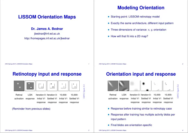
Orientation input and response

Retinal activation LGN response Iteration 0: Initial V1 response Iteration 0: Settled V1 response 10,000: Initial V1 response 10,000: Settled V1 response

CMVC figure 5.6

  • Response before training similar to retinotopy case
  • Response after training has multiple activity blobs per

input pattern

  • Final blobs are orientation-specific

CNV Spring 2015: LISSOM Orientation Maps 4

slide-2
SLIDE 2

Self-organized V1 weights

Afferent (ON−OFF) Lateral excitatory Lateral inhibitory

CMVC figure 5.7

Typical:

  • Gabor-like afferent CF
  • Nearly uniform short-range lateral excitatory
  • Patchy, orientation-specific long-range lateral inhibitory

CNV Spring 2015: LISSOM Orientation Maps 5

Self-organized weights across V1

Afferent (ON−OFF) Lateral inhibitory

CMVC figure 5.8

CNV Spring 2015: LISSOM Orientation Maps 6

OR map self-organization

Iteration 0 Iteration 10,000

OR preference OR selectivity OR preference & selectivity OR H

CMVC figure 5.9

CNV Spring 2015: LISSOM Orientation Maps 7

Macaque ORmap: Fourier,gradient

Fourier spectrum Gradient

CMVC figure 5.1

In monkeys:

  • Ring-shaped spectrum:

repeats regularly in all directions

  • High gradient at fractures, pinwheels.

CNV Spring 2015: LISSOM Orientation Maps 8

slide-3
SLIDE 3

OR Map: Fourier, gradient

Fourier spectrum Gradient

CMVC figure 5.10

LISSOM model has similar spectrum, gradient

CNV Spring 2015: LISSOM Orientation Maps 9

OR Map: Retinotopic organization

CMVC figure 5.11

  • Retinotopy is distorted locally by orientation prefs
  • Matches distortions found in animal maps?

CNV Spring 2015: LISSOM Orientation Maps 10

OR Map: Lateral connections

OR weights OR CH OR connections

Connections in iso-OR patches Connections in OR pinwheels Connections in OR saddles Connections in OR fractures

CMVC figure 5.12

CNV Spring 2015: LISSOM Orientation Maps 11

Effect of initial weights

Weights 2 Weights 1 (a) Iteration 0 (b) Iteration 50 (c) Iteration 10,000

CMVC figure 8.5

Changing weights doesn’t change map folding pattern.

CNV Spring 2015: LISSOM Orientation Maps 12

slide-4
SLIDE 4

Effect of input streams

Inputs 1 Inputs 2 (a) Iteration 0 (b) Iteration 50 (c) Iteration 10,000

CMVC figure 8.5

Changing inputs changes entire pattern.

CNV Spring 2015: LISSOM Orientation Maps 13

Scaling retinal and cortical area

(a) Original retina: R = 24 (b) Retinal area scaled by 4.0:

R = 96

CMVC figure 15.1a,b

CNV Spring 2015: LISSOM Orientation Maps 14

Scaling retinal and cortical area

(c) Original V1:

N = 54, 0.4 hours, 8 MB

(d) V1 area scaled by 4.0:

N = 216, 9 hours, 148 MB

CMVC figure 15.1c,d

CNV Spring 2015: LISSOM Orientation Maps 15

Scaling retinal density

Retina V1 Original retina Retina scaled by 2 Retina scaled by 3

CMVC figure 15.2

CNV Spring 2015: LISSOM Orientation Maps 16

slide-5
SLIDE 5

Scaling cortical density

(a)

36 × 36:

0.17 hours, 2.0 MB (b)

48 × 48:

0.32 hours, 5.2 MB (c)

72 × 72:

0.77 hours, 22 MB (d)

96 × 96:

1.73 hours, 65 MB (e)

144×144:

5.13 hours, 317 MB

CMVC figure 15.3

Above minimum density (due to lateral radii), density not crucial for organization

CNV Spring 2015: LISSOM Orientation Maps 17

Full-size V1 Map

  • Map scaled to

cover most of visual field

  • Allows testing

with full-size images

  • 30 million

connections

CNV Spring 2015: LISSOM Orientation Maps 18

Sample Image

CNV Spring 2015: LISSOM Orientation Maps 19

RGC/LGN Response

CNV Spring 2015: LISSOM Orientation Maps 20

slide-6
SLIDE 6

V1 Response with γn

CNV Spring 2015: LISSOM Orientation Maps 21

V1 Orientation Map

CNV Spring 2015: LISSOM Orientation Maps 22

Afferent normalization

LISSOM mechanism for contrast invariant tuning:

sij = γA @ X

ρab

ξρabAρab,ij 1 A 1 + γn @ X

ρab

ξρab 1 A ,

(1)

ξρab: activation of unit (a, b) in afferent CF ρ of neuron (i, j) Aab,ij is the corresponding afferent weight γA, γn are constant scaling factors

GCAL achieves similar results with lateral inhibition in RGC/LGN

CNV Spring 2015: LISSOM Orientation Maps 23

RGC/LGN response to large image

Retinal activation LGN response

CMVC figure 8.2a,b

RGC/LGN responds to most of the visible contours

CNV Spring 2015: LISSOM Orientation Maps 24

slide-7
SLIDE 7

V1 without afferent normalization

V1 response:

γn = 0, γA = 3.25

V1 response:

γn = 0, γA = 7.5

CMVC figure 8.2c-e

Cannot get selective response to all contours

CNV Spring 2015: LISSOM Orientation Maps 25

V1 with afferent normalization

V1 response:

γn = 0, γA = 3.25

V1 response:

γn = 80, γA = 30

CMVC figure 8.2c-e

Responds based on contour, not contrast

CNV Spring 2015: LISSOM Orientation Maps 26

Tuning with afferent normalization

  • 30
  • 60
  • 90
  • 120
  • 150
  • Orientation

0.0 0.2 0.4 0.6 0.8 1.0 Peak settled response

γn = 0, γA = 3.25

  • 30
  • 60
  • 90
  • 120
  • 150
  • Orientation

0.0 0.2 0.4 0.6 0.8 1.0 Peak settled response 100% 90% 80% 70% 60% 50% 40% 30% 20% 10%

γn = 80, γA = 30

CMVC figure 8.3

Sine grating tuning curve:

  • Without γn: selectivity lost as contrast increases
  • With γn: always orientation-specific

CNV Spring 2015: LISSOM Orientation Maps 27

OR Map: Gaussian

CMVC figure 5.13

Retina LGN RFs LIs ORpref.&sel. OR H OR FFT

White line CFs only

CNV Spring 2015: LISSOM Orientation Maps 28

slide-8
SLIDE 8

OR Map: +/- Gaussian

CMVC figure 5.13

Retina LGN RFs LIs ORpref.&sel. OR H OR FFT

White or black line CFs OR map disrupted due to phase columns

CNV Spring 2015: LISSOM Orientation Maps 29

OR Map: Retinal wave model

CMVC figure 5.13

Retina LGN RFs LIs ORpref.&sel. OR H OR FFT

Some line, mostly edge CFs

CNV Spring 2015: LISSOM Orientation Maps 30

OR Map: Smooth disks

CMVC figure 5.13

Retina LGN RFs LIs ORpref.&sel. OR H OR FFT

All edge CFs

CNV Spring 2015: LISSOM Orientation Maps 31

OR Map: Natural images

CMVC figure 5.13

Retina LGN RFs LIs ORpref.&sel. OR H OR FFT

All types of CFs Longer range lateral weights Histogram: horizontal, vertical bias

CNV Spring 2015: LISSOM Orientation Maps 32

slide-9
SLIDE 9

OR Map: Uniform noise

CMVC figure 5.13

Retina LGN RFs LIs ORpref.&sel. OR H OR FFT

Relatively unselective CFs

CNV Spring 2015: LISSOM Orientation Maps 33

Modeling pre/post-natal phases

Input patterns

1000 5000 10000

  • Prenatal: internal activity
  • Postnatal: natural images (Shouval et al. 1996)

CNV Spring 2015: LISSOM Orientation Maps 34

Pre/post-natal V1 development

Input patterns Orientation maps

1000 5000 10000

  • Neonatal map smoothly becomes more selective

CNV Spring 2015: LISSOM Orientation Maps 35

Statistics drive development

Input patterns Orientation maps

1000 5000 10000

  • Biased image dataset: mostly landscapes
  • Smoothly changes into horizontal-dominated map

CNV Spring 2015: LISSOM Orientation Maps 36

slide-10
SLIDE 10

OR Histograms

0◦ 90◦ 180◦

HLISSOM model

0◦ 90◦ 180◦

Adult ferret V1

(Coppola et al. 1998)

  • After postnatal training on Shouval natural images,
  • rientation histogram matches results from ferrets
  • Model adapts to statistical structure of images

CNV Spring 2015: LISSOM Orientation Maps 37

Stable development

(Stevens et al. 2013) L GCAL Ferret

GCAL map development is stable like ferret V1; LISSOM is unstable even w/o threshold changes, radius shrinking (L)

CNV Spring 2015: LISSOM Orientation Maps 38

Pinwheel density

(Stevens et al. 2013)

  • Animal orientation maps have an average of π

pinwheels per hypercolumn (Kaschube et al. 2010)

  • GCAL is so far the only mechanistic model shown to

have this property

  • LISSOM probably would as well, but requires

unrealistic mechanisms to do so, since L does not

CNV Spring 2015: LISSOM Orientation Maps 39

Summary

  • Development depends on features of input pattern
  • Orientation maps develop with many different patterns
  • Develops Gabor-type CFs with most inputs
  • Breaks up image into oriented patches
  • Scale response by local contrast to work for large images
  • Matching biology requires prenatal, postnatal phases
  • Can get more elaborate: complex cells, multiple

laminae/cell types, short-range inhibition, feedback, ...

CNV Spring 2015: LISSOM Orientation Maps 40

slide-11
SLIDE 11

References

Coppola, D. M., White, L. E., Fitzpatrick, D., & Purves, D. (1998). Unequal repre- sentation of cardinal and oblique contours in ferret visual cortex. Proceed- ings of the National Academy of Sciences, USA, 95 (5), 2621–2623. Kaschube, M., Schnabel, M., L¨

  • wel, S., Coppola, D. M., White, L. E., & Wolf, F.

(2010). Universality in the evolution of orientation columns in the visual

  • cortex. Science, 330 (6007), 1113–1116.

Miikkulainen, R., Bednar, J. A., Choe, Y., & Sirosh, J. (2005). Computational Maps in the Visual Cortex. Berlin: Springer. Shouval, H. Z., Intrator, N., Law, C. C., & Cooper, L. N. (1996). Effect of binoc- ular cortical misalignment on ocular dominance and orientation selectivity. Neural Computation, 8 (5), 1021–1040.

CNV Spring 2015: LISSOM Orientation Maps 40

Stevens, J.-L. R., Law, J. S., Antolik, J., & Bednar, J. A. (2013). Mechanisms for stable, robust, and adaptive development of orientation maps in the primary visual cortex. Journal of Neuroscience, 33, 15747–15766.

CNV Spring 2015: LISSOM Orientation Maps 40