Modeling of Survival Data Now we will explore the relationship - - PowerPoint PPT Presentation

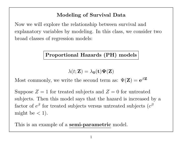
Modeling of Survival Data Now we will explore the relationship between survival and explanatory variables by modeling. In this class, we consider two broad classes of regression models: Proportional Hazards (PH) models λ(t; Z) = λ0(t)Ψ(Z) Most commonly, we write the second term as: Ψ(Z) = eβZ Suppose Z = 1 for treated subjects and Z = 0 for untreated

• subjects. Then this model says that the hazard is increased by a

factor of eβ for treated subjects versus untreated subjects (cβ might be < 1). This is an example of a semi-parametric model.

1

Accelerated Failure Time (AFT) models log(T) = µ + βZ + σw where w is an “error distribution”. Typically, we place a parametric assumption on w:

• exponential, Weibull, Gamma
• lognormal

Covariates In general, Z is a vector of covariates of interest. Z may include:

• continuous factors (eg, age, blood pressure)
• discrete factors (gender, marital status)
• possible interactions (age by sex interaction)

2

Covariates Just as in standard linear regression, if we have a discrete covariate A with a levels, then we will need to include (a − 1) dummy variables (U1, U2, . . . , Ua) such that Uj = 1 if A = j. Then λi(t) = λ0(t) exp(β2U2 + β3U3 + · · · + βaUa) (In the above model, the subgroup with A = 1 or U1 = 1 is the reference group.) Interactions Two factors, A and B, interact if the hazard of death depends on the combination of levels of A and B. We follow the principle of hierarchical models, and only include interactions if all of the associated main effects are also included.

3

The example I just gave was based on a proportional hazards model, but the description of the types of covariates we might want to include in our model applies to both the AFT and PH model. We’ll start out by focusing on the Cox PH model, and address some of the following questions:

• What does the term λ0(t) mean?
• What’s “proportional” about the PH model?
• How do we estimate the parameters in the model?
• How do we interpret the estimated values?
• How can we construct tests of whether the covariates have a

significant effect on the distribution of survival times?

• How do these tests compare to the logrank test or the

Wilcoxon test?

4

The Cox Proportional Hazards model λ(t; Z) = λ0(t) exp(βZ)

This is the most common model used for survival data. Why?

• flexible choice of covariates
• fairly easy to fit
• standard software exists

References: Collett, Chapter 3 Allison, Chapter 5 Cox and Oakes, Chapter 7 Kleinbaum, Chapter 3 Klein and Moeschberger, Chapters 8 & 9 Kalbfleisch and Prentice Lee

5

Some books (like Collett) use h(t; X) as their standard notation instead of λ(t; Z). Why do we call it proportional hazards? Think of the first example, where Z = 1 for treated and Z = 0 for

• control. Then if we think of λ1(t) as the hazard rate for the treated

group, and λ0(t) as the hazard for control, then we can write: λ1(t) = λ(t; Z = 1) = λ0(t) exp(βZ) = λ0(t) exp(β) This implies that the ratio of the two hazards is a constant, φ, which does NOT depend on time, t. In other words, the hazards of the two groups remain proportional over time. φ = λ1(t) λ0(t) = eβ φ is referred to as the hazard ratio. What is the interpretation of β here?

6

The Baseline Hazard Function In the example of comparing two treatment groups, λ0(t) is the hazard rate for the control group. In general, λ0(t) is called the baseline hazard function, and reflects the underlying hazard for subjects with all covariates Z1, ..., Zp equal to 0 (i.e., the ”reference group”). The general form is: λ(t; Z) = λ0(t) exp(β1Z1 + β2Z2 + · · · + βpZp) So when we substitute all of the Zj’s equal to 0, we get: λ(t, Z = 0) = λ0(t) exp(β1 ∗ 0 + β2 ∗ 0 + · · · + βp ∗ 0) = λ0(t) In the general case, we think of the i-th individual having a set of covariates Zi = (Z1i, Z2i, ..., Zpi), and we model their hazard rate

7

as some multiple of the baseline hazard rate: λi(t, Zi) = λ0(t) exp(β1Z1i + · · · + βpZpi) This means we can write the log of the hazard ratio for the i-th individual to the reference group as: log λi(t) λ0(t)

• =

β1Z1i + β2Z2i + · · · + βpZpi The Cox Proportional Hazards model is a linear model for the log of the hazard ratio

8

One of the biggest advantages of the framework of the Cox PH model is that we can estimate the parameters β which reflect the effects of treatment and other covariates without having to make any assumptions about the form of λ0(t). In other words, we don’t have to assume that λ0(t) follows an exponential model, or a Weibull model, or any other particular parametric model. That’s what makes the model semi-parametric. Questions:

• 1. Why don’t we just model the hazard ratio,

φ = λi(t)/λ0(t), directly as a linear function of the covariates Z?

• 2. Why doesn’t the model have an intercept?

9

Estimation of the model parameters The basic idea is that under PH, information about β can be

• btained from the relative orderings (i.e., ranks) of the survival

times, rather than the actual values. Why? Suppose T follows a PH model: λ(t; Z) = λ0(t)eβZ Now consider T ∗ = g(T), where g is a monotonic increasing

• function. We can show that T ∗ also follows the PH model, with the

same multiplier, eβZ. Therefore, when we consider likelihood methods for estimating the model parameters, we only have to worry about the ranks of the survival times.

10

Likelihood Estimation for the PH Model Kalbfleisch and Prentice derive a likelihood involving only β and Z (not λ0(t)) based on the marginal distribution of the ranks of the

• bserved failure times (in the absence of censoring).

Cox (1972) derived the same likelihood, and generalized it for censoring, using the idea of a partial likelihood Suppose we observe (Xi, δi, Zi) for individual i, where

• Xi is a censored failure time random variable
• δi is the failure/censoring indicator (1=fail,0=censor)
• Zi represents a set of covariates

The covariates may be continuous, discrete, or time-varying.

11

Suppose there are K distinct failure (or death) times, and let τ1, ....τK represent the K ordered, distinct death times. For now, assume there are no tied death times. Let R(t) = {i : xi ≥ t} denote the set of individuals who are “at risk” for failure at time t. More about risk sets:

• I will refer to R(τj) as the risk set at the jth failure time
• I will refer to R(Xi) as the risk set at the failure time of

individual i

• There will still be rj individuals in R(τj).
• rj is a number, while R(τj) identifies the actual subjects at risk

12

What is the partial likelihood? Intuitively, it is a product over the set of observed death times of the conditional probabilities of seeing the observed deaths, given the set of individuals at risk at those times. At each death time τj, the contribution to the likelihood is: Lj(β) = Pr(individual j fails|1 failure from R(τj)) = Pr(individual j fails| at risk at τj)

• ℓ∈R(τj) Pr(individual ℓ fails| at risk at τj)

= λ(τj; Zj)

• ℓ∈R(τj) λ(τj; Zℓ)

13

Under the PH assumption, λ(t; Z) = λ0(t)eβZ, so we get: Lpartial(β) =

K

• j=1

λ0(τj)eβZj

• ℓ∈R(τj) λ0(τj)eβZℓ

=

K

• j=1

eβZj

• ℓ∈R(τj) eβZℓ

14

Another derivation: In general, the likelihood contributions for censored data fall into two categories:

• Individual is censored at Xi:

Li(β) = S(Xi) = exp[− Xi λi(u)du]

• Individual fails at Xi:

Li(β) = S(Xi)λi(Xi) = λi(Xi) exp[− Xi λi(u)du] Thus, everyone contributes S(Xi) to the likelihood, and only those who fail contribute λi(Xi).

15

This means we get a total likelihood of: L(β) =

n

• i=1

λi(Xi)δi exp[− Xi λi(u)du] The above likelihood holds for all censored survival data, with general hazard function λ(t). In other words, we haven’t used the Cox PH assumption at all yet. Now, let’s multiply and divide by the term

• j∈R(Xi) λi(Xi)

δi :

L(β) =

n

• i=1
• λi(Xi)
• j∈R(Xi) λi(Xi)

δi  

• j∈R(Xi)

λi(Xi)  

δi

exp[− Xi λi(u)du]

Cox (1972) argued that the first term in this product contained almost all of the information about β, while the second two terms contained the information about λ0(t), i.e., the baseline hazard.

16

If we just focus on the first term, then under the Cox PH assumption: L(β) =

n

• i=1
• λi(Xi)
• j∈R(Xi) λi(Xi)

δi =

n

• i=1
• λ0(Xi) exp(βzi)
• j∈R(Xi) λ0(Xi) exp(βzj)

δi =

n

• i=1
• exp(βzi)
• j∈R(Xi) exp(βzj)

δi This is the partial likelihood defined by Cox. Note that it does not depend on the underlying hazard function λ0(·). Cox recommends treating this as an ordinary likelihood for making inferences about β in the presence of the nuisance parameter λ0(·).

17

A simple example: individual Xi δi Zi 1 9 1 4 2 8 5 3 6 1 7 4 10 1 3 Now let’s compile the pieces that go into the partial likelihood contributions at each failure time:

18

• rdered

failure Likelihood contribution j time Xi R(Xi) ij

• eβZi/

j∈R(Xi) eβZj

δi 1 6 {1,2,3,4} 3 e7β/[e4β + e5β + e7β + e3β] 2 8 {1,2,4} 2 1 3 9 {1,4} 1 e4β/[e4β + e3β] 4 10 {4} 4 e3β/e3β = 1 The partial likelihood would be the product of these four terms.

19

Notes on the partial likelihood L(β) =

n

• j=1
• eβzj
• ℓ∈R(Xj) eβzℓ

δj =

K

• j=1

eβZj

• ℓ∈R(τj) eβZℓ

where the product is over the K death (or failure) times.

• contributions only at the death times
• the partial likelihood is NOT a product of independent terms,

but of conditional probabilities

• There are other choices besides Ψ(z) = eβz, but this is the most

common and the one for which software is generally available.

20

Partial Likelihood inference Inference can be conducted by treating the partial likelihood as though it satisfied all the regular likelihood properties (take the more advanced failure time course to see why!!) The log-partial likelihood is

ℓ(β) = log n

• j=1

eβzj

• ℓ∈R(Xj) eβzℓ

δj = log K

• j=1

eβzj

• ℓ∈R(τj) eβzℓ
• =

K

• j=1

 βzj − log[

• ℓ∈R(τj)

eβzℓ]   =

K

• j=1

lj(β)

where lj is the log-partial likelihood contribution at the j-th

• rdered death time.

21

Suppose there is only one covariate (β is one-dimensional). The partial likelihood score equations are: U(β) = ∂ ∂β ℓ(β) =

n

• j=1

δj

• Zj −
• ℓ∈R(Xj) ZℓeβZℓ
• ℓ∈R(Xj) eβZℓ
• We can express U(β) intuitively as a sum of “observed” minus

“expected” values: U(β) = ∂ ∂β ℓ(β) =

n

• j=1

δj(Zj − ¯ Zj) where ¯ Zj is the “weighted average” of the covariate Z over all the individuals in the risk set at time τj. Note that β is involved through the term ¯ Zj. The maximum partial likelihood estimators can be found by solving U(β) = 0.

22

Like standard likelihood theory, it can be shown (not easily) that ( β − β) se(ˆ β) ∼ N(0, 1) The variance of ˆ β can be obtained by inverting the second derivative of the partial likelihood, var(ˆ β) ∼

• − ∂2

∂β2 ℓ(β) −1 From the above expression for U(β), we have: ∂2 ∂β2 ℓ(β) =

n

• j=1

δj

• −
• ℓ∈R(τj)(Zj − ¯

Zj)2eβZℓ

• ℓ∈R(τj) eβZℓ
• Note: The true variance of ˆ

β is a function of the unknown β. We calculate the “observed” information by substituting the partial likelihood estimate of β into the above variance formula.

23

Simple Example for 2-group comparison: (no ties)

Group 0: 4+, 7, 8+, 9, 10+ = ⇒ Zi = 0 Group 1: 3, 5, 5+, 6, 8+ = ⇒ Zi = 1

• rdered failure

Number at risk Likelihood contribution j time Xi Group 0 Group 1

• eβZi/

j∈R(Xi) eβZj

δi 1 3 5 5 eβ/[5 + 5eβ] 2 5 4 4 eβ/[4 + 4eβ] 3 6 4 2 eβ/[4 + 2eβ] 4 7 4 1 e0/[4 + 1eβ] = 1/[4 + eβ] 5 9 2 e0/[2 + 0] = 1/2 Again, we take the product over the likelihood contributions, then maximize to get the partial MLE for β. What does β represent in this case?

24

Notes

• The “observed” information matrix is generally used because in

practice, people find it has better properties. Also, the “expected” is very hard to calculate.

• There is a nice analogy with the score and information

matrices from more standard regression problems, except that here we are summing over observed death times, rather than individuals.

• Newton Raphson is used by many of the computer packages to

solve the partial likelihood equations.

25

Fitting Cox PH model with Stata STATA uses the “stcox” command. First, try typing “help stcox”

• help for stcox
• Estimate Cox proportional hazards model
• stcox [varlist] [if exp] [in range]

[, nohr strata(varnames) robust cluster(varname) noadjust mgale(newvar) esr(newvars) schoenfeld(newvar) scaledsch(newvar) basehazard(newvar) basechazard(newvar) basesurv(newvar) {breslow | efron | exactm | exactp} cmd estimate noshow

• ffset level(#) maximize-options ]

stphtest [, km log rank time(varname) plot(varname) detail graph-options ksm-options] 26

stcox is for use with survival-time data; see help st. You must have stset your data before using this command; see help stset. Description

• stcox estimates maximum-likelihood proportional hazards models on st data.

Options (many more!)

• nohr reports the estimated coefficients rather than hazard ratios; i.e.,

b rather than exp(b). Standard errors and confidence intervals are similarly transformed. This option affects how results are displayed, not how they are estimated. 27

Example Leukemia Data

. stcox trt Iteration 0: log likelihood =

• 93.98505

Iteration 1: log likelihood = -86.385606 Iteration 2: log likelihood = -86.379623 Iteration 3: log likelihood = -86.379622 Refining estimates: Iteration 0: log likelihood = -86.379622 Cox regression -- Breslow method for ties

• No. of subjects =

42 Number of obs = 42

• No. of failures =

30 Time at risk = 541 LR chi2(1) = 15.21 Log likelihood =

• 86.379622

Prob > chi2 = 0.0001

• _t |

_d | Haz. Ratio

• Std. Err.

z P>|z| [95% Conf. Interval]

• --------+--------------------------------------------------------------------

trt | .2210887 .0905501

• 3.685

0.000 .0990706 .4933877

• 28

. stcox trt , nohr Iteration 0: log likelihood =

• 93.98505

Iteration 1: log likelihood = -86.385606 Iteration 2: log likelihood = -86.379623 Iteration 3: log likelihood = -86.379622 Refining estimates: Iteration 0: log likelihood = -86.379622 Cox regression -- Breslow method for ties

• No. of subjects =

42 Number of obs = 42

• No. of failures =

30 Time at risk = 541 LR chi2(1) = 15.21 Log likelihood =

• 86.379622

Prob > chi2 = 0.0001

• _t |

_d | Coef.

• Std. Err.

z P>|z| [95% Conf. Interval]

• --------+--------------------------------------------------------------------

trt |

• 1.509191

.4095644

• 3.685

0.000

• 2.311923
• .7064599
• 29

More Notes:

• The Cox Proportional hazards model has the advantage over a

simple logrank test of giving us an estimate of the “risk ratio” (i.e., φ = λ1(t)/λ0(t)). This is more informative than just a test statistic, and we can also form confidence intervals for the risk ratio.

• In this case, ˆ

φ = 0.221, which can be interpreted to mean that the hazard for relapse among patients treated with 6-MP is less than 25% of that for placebo patients.

• From the sts list command in Stata or Proc lifetest in

SAS, we were able to get estimates of the entire survival distribution ˆ S(t) for each treatment group; we can’t immediately get this from our Cox model without further

• assumptions. Why not?

30

Adjustments for ties The proportional hazards model assumes a continuous hazard – ties are not possible. There are four proposed modifications to the likelihood to adjust for ties. (1) Cox’s (1972) modification: “discrete” method (2) Peto-Breslow method (3) Efron’s (1977) method (4) Exact method (Kalbfleisch and Prentice) (5) Exact marginal method

31

Some notation: τ1, ....τK the K ordered, distinct death times dj the number of failures at τj Hj the “history” of the entire data set, up to the j-th death or failure time, including the time

• f the failure, but not the identities of the dj

who fail there. ij1, ...ijdj the identities of the dj individuals who fail at τj

32

Cox’s (1972) modification: “discrete” method Cox’s method assumes that if there are tied failure times, they truly happened at the same time. It is based on a discrete likelihood. The partial likelihood is:

L(β) =

K

• j=1

Pr(ij1, ...ijdj fail | dj fail at τj, from R) =

K

• j=1

Pr(ij1, ...ijdj fail | in R(τj))

• ℓ∈s(j,dj) Pr(ℓ1, ....ℓdj fail | in R(τj))

=

K

• j=1

exp(βzij1) · · · exp(βzijdj )

• ℓ∈s(j,dj) exp(βzℓ1) · · · exp(βzℓdj )

=

K

• j=1

exp(βSj)

• ℓ∈s(j,dj) exp(βSjℓ)

33

In the previous formula

• s(j, dj) is the set of all possible sets of dj individuals that can

possibly be drawn from the risk set at time τj

• Sj is the sum of the Z’s for all the dj individuals who fail at τj
• Sjℓ is the sum of the Z’s for all the dj individuals in the ℓ-th

set drawn out of s(j, dj)

34

What does this all mean??!! Let’s modify our previous simple example to include ties.

Simple Example (with ties) Group 0: 4+, 6, 8+, 9, 10+ = ⇒ Zi = 0 Group 1: 3, 5, 5+, 6, 8+ = ⇒ Zi = 1

Ordered failure Number at risk

• Lik. Contribution

j time Xi Group 0 Group 1 eβSj /

ℓ∈s(j,dj ) eβSjℓ

1 3 5 5 eβ/[5 + 5eβ] 2 5 4 4 eβ/[4 + 4eβ] 3 6 4 2 eβ/[6 + 8eβ + e2β] 4 9 2 e0/2 = 1/2 35

The tie occurs at t = 6, when R(τj) = {Z = 0 : (6, 8+, 9, 10+), Z = 1 : (6, 8+)}. Of the 6

2

• = 15 possible pairs of subjects at risk

at t=6, there are 6 pairs formed where both are from group 0 (Sj = 0), 8 pairs formed with one in each group (Sj = 1), and 1 pairs formed with both in group 1 (Sj = 2). Problem: With numbers of ties, the denominator can have many many terms and be difficult to calculate.

36

Breslow method: (default) Breslow and Peto suggested replacing the term

ℓ∈s(j,dj) eβSjℓ in

the denominator by the term

• ℓ∈R(τj) eβZℓ

dj , so that the following modified partial likelihood would be used: L(β) =

K

• j=1

eβSj

• ℓ∈s(j,dj) eβSjℓ ≈

K

• j=1

eβSj

• ℓ∈R(τj) eβZℓ

dj

37

Justification: Suppose individuals 1 and 2 fail from {1, 2, 3, 4} at time τj. Let φ(i) be the hazard ratio for individual i (compared to baseline).

eβSj

• ℓ∈s(j,dj) eβSjℓ

= φ(1) φ(1) + φ(2) + φ(3) + φ(4) × φ(2) φ(2) + φ(3) + φ(4) + φ(2) φ(1) + φ(2) + φ(3) + φ(4) × φ(1) φ(1) + φ(3) + φ(4) ≈ 2φ(1)φ(2) [φ(1) + φ(2) + φ(3) + φ(4)]2 The Peto (Breslow) approximation will break down when the number of ties are relative to the size of the risk sets, and then tends to yield estimates of β which are biased toward 0.

38

Efron’s (1977) method: Efron suggested an even closer approximation to the discrete likelihood: L(β) =

K

• j=1

eβSj

• ℓ∈R(τj) eβZℓ + j−1

dj

• ℓ∈D(τj) eβZℓ

dj Like the Breslow approximation, Efron’s method will yield estimates of β which are biased toward 0 when there are many ties. However, (1995) Allison recommends the Efron approximation since it is much faster than the exact methods and tends to yield much closer estimates than the default Breslow approach.

39

Exact method (Kalbfleisch and Prentice) The “discrete” option that we discussed in (1) is an exact method based on a discrete likelihood (assuming that tied events truly ARE tied). This second exact method is based on the continuous likelihood, under the assumption that if there are tied events, that is due to the imprecise nature of our measurement, and that there must be some true ordering. All possible orderings of the tied events are calculated, and the probabilites of each are summed.

40

Example with 2 tied events (1,2) from riskset (1,2,3,4):

eβSj

• ℓ∈s(j,dj) eβSjℓ

= eβS1 eβS1 + eβS2 + eβS3 + eβS4 × eβS2 eβS2 + eβS3 + eβS4 + eβS2 eβS1 + eβS2 + eβS3 + eβS4 × eβS1 eβS1 + eβS3 + eβS4

41

Bottom Line Implications of Ties (See Allison (1995), p.127-137) (1) When there are no ties, all four options give exactly the same results. (2) When there are only a few ties, it won’t make much difference which method is used. However, since the exact methods won’t take much extra computing time, you might as well use one of them. (3) When there are many ties (relative to the number at risk), the Breslow option (default) performs poorly (Farewell & Prentice, 1980; Hsieh, 1995). Both of the approximate methods, Breslow and Efron, yield coefficients that are attenuated (biased toward 0).

42

(4) The choice of which exact method to use should be based

• n substantive grounds - are the tied event times truly tied?

...or are they the result of imprecise measurement? (5) Computing time of exact methods is much longer than that of the approximate methods. However, in most cases it will still be less than 30 seconds even for the exact methods. (6) Best approximate method - the Efron approximation nearly always works better than the Breslow method, with no increase in computing time, so use this option if exact methods are too computer-intensive.

43

Stata Commands for PH Model with Ties: Stata offers four options for adjustments with tied data:

• breslow (default)
• efron
• exactp (same as the “discrete” option in SAS)
• exactm - an exact marginal likelihood calculation

(different than the “exact” option in SAS)

44

Fecundability Data Example:

. stcox smoker, efron nohr failure _d: status analysis time _t: cycle Iteration 0: log likelihood = -3113.5313 Iteration 1: log likelihood = -3107.3102 Iteration 2: log likelihood = -3107.2464 Iteration 3: log likelihood = -3107.2464 Refining estimates: Iteration 0: log likelihood = -3107.2464 Cox regression -- Efron method for ties

• No. of subjects =

586 Number of obs = 586

• No. of failures =

567 Time at risk = 1844 LR chi2(1) = 12.57 Log likelihood =

• 3107.2464

Prob > chi2 = 0.0004

• _t |

_d | Coef.

• Std. Err.

z P>|z| [95% Conf. Interval]

• --------+--------------------------------------------------------------------

smoker |

• .3877931

.1140202

• 3.401

0.001

• .6112685
• .1643177
• 45

A special case: the two-sample problem Previously, we derived the logrank test from an intuitive perspective, assuming that we have (X01, δ01) . . . (X0n0, δ0n0) from group 0 and (X11, δ11), . . . , (X1n1, δ1n1) from group 1. Just as a χ2 test for binary data can be derived from a logistic model, we will see here that the logrank test can be derived as a special case of the Cox Proportional Hazards model. First, let’s re-define our notation in terms of (Xi, δi, Zi):

(X01, δ01), . . . , (X0n0, δ0n0) = ⇒ (X1, δ1, 0), . . . , (Xn0, δn0, 0) (X11, δ11), . . . , (X1n1, δ1n1) = ⇒ (Xn0+1, δn0+1, 1), . . . , (Xn0+n1, δn0+n1, 1)

In other words, we have n0 rows of data (Xi, δi, 0) for the group 0 subjects, then n1 rows of data (Xi, δi, 1) for the group 1 subjects.

46

Using the proportional hazards formulation, we have λ(t; Z) = λ0(t) eβZ Group 0 hazard: λ0(t) Group 1 hazard: λ0(t) eβ The log-partial likelihood is: logL(β) = log  

K

• j=1

eβZj

• ℓ∈R(τj) eβZℓ

  =

K

• j=1

 βZj − log[

• ℓ∈R(τj)

eβZℓ]  

47

Taking the derivative with respect to β, we get: U(β) = ∂ ∂β ℓ(β) =

n

• j=1

δj

• Zj −
• ℓ∈R(τj) ZℓeβZℓ
• ℓ∈R(τj) eβZℓ
• =

n

• j=1

δj(Zj − ¯ Zj) where ¯ Zj =

• ℓ∈R(τj) ZℓeβZℓ
• ℓ∈R(τj) eβZℓ

U(β) is called the “score”.

48

As we discussed earlier in the class, one useful form of a likelihood-based test is the score test. This is obtained by using the score U(β) evaluated at Ho as a test statistic. Let’s look more closely at the form of the score: δjZj

• bserved number of deaths in group 1 at τj

δj ¯ Zj expected number of deaths in group 1 at τj Why? Under H0 : β = 0, ¯ Zj is simply the number of individuals from group 1 in the risk set at time τj (call this r1j), divided by the total number in the risk set at that time (call this rj). Thus, ¯ Zj approximates the probability that given there is a death at τj, it is from group 1.

49

Thus, the score statistic is of the form:

n

• j=1

(Oj − Ej) When there are ties, the likelihood has to be replaced by one that allows for ties. In Stata: discrete/exactp → Mantel-Haenszel logrank test breslow → linear rank version of the logrank test

50