Comparison of Survival Curves We spent the last class looking at - - PowerPoint PPT Presentation

Comparison of Survival Curves We spent the last class looking at some nonparametric approaches for estimating the survival function, ˆ S(t), over time for a single sample of individuals. Now we want to compare the survival estimates between two groups.

1

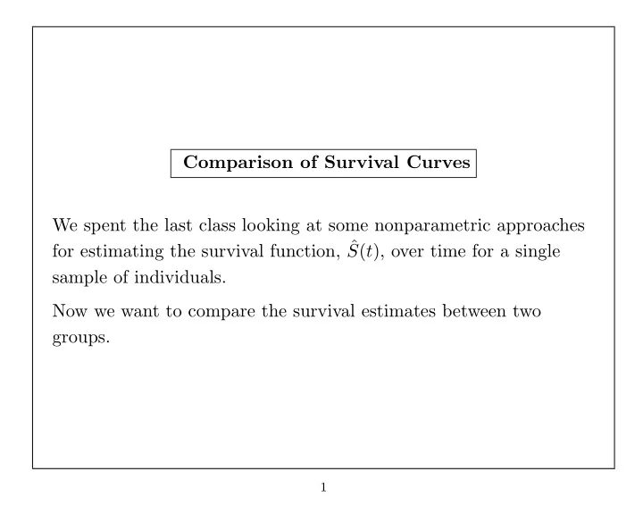
Example: Time to remission of leukemia patients

0.00 0.25 0.50 0.75 1.00 10 20 30 40 analysis time trt = Control trt = 6MP

Estimated survival probability 2

How can we form a basis for comparison? At a specific point in time, we could see whether the confidence intervals for the survival curves overlap. However, the confidence intervals we have been calculating are “pointwise” ⇒ they correspond to a confidence interval for ˆ S(t∗) at a single point in time, t∗. In other words, we can’t say that the true survival function S(t) is contained between the pointwise confidence intervals with 95% probability. (Aside: if you’re interested, the issue of confidence bands for the estimated survival function are discussed in Section 4.4 of Klein and Moeschberger)

3

Looking at whether the confidence intervals for ˆ S(t∗) overlap between the 6MP and placebo groups would only focus on comparing the two treatment groups at a single point in time, t∗. Should we base our overall comparison of ˆ S(t) on:

• the furthest distance between the two curves?
• the median survival for each group?
• the average hazard? (for exponential distributions, this would be

like comparing the mean event times)

• adding differences between the two survival estimates over time?

X

j

h ˆ S(tjA) − ˆ S(tjB) i

• a weighted sum of differences, where the weights reflect the number

at risk at each time?

• a rank-based test? i.e., we could rank all of the event times, and then

see whether the sum of ranks for one group was less than the other.

4

Nonparametric comparisons of groups All of these are pretty reasonable options, and we’ll see that there have been several proposals for how to compare the survival of two

• groups. For the moment, we are sticking to nonparametric

comparisons. Why nonparametric?

• fairly robust
• efficient relative to parametric tests
• often simple and intuitive

Before continuing the description of the two-sample comparison, I’m going to try to put this in a general framework to give a perspective of where we’re heading in this class.

5

General Framework for Survival Analysis We observe (Xi, δi, Zi) for individual i, where

• Xi is a censored failure time random variable
• δi is the failure/censoring indicator
• Zi represents a set of covariates

Note that Zi might be a scalar (a single covariate, say treatment or gender) or may be a (p × 1) vector (representing several different covariates).

6

These covariates might be:

• continuous
• discrete
• time-varying (more later)

If Zi is a scalar and is binary, then we are comparing the survival

• f two groups, like in the leukemia example.

More generally though, it is useful to build a model that characterizes the relationship between survival and all of the covariates of interest.

7

We’ll proceed as follows:

• Two group comparisons
• Multigroup and stratified comparisons - stratified logrank
• Failure time regression models

– Cox proportional hazards model – Accelerated failure time model

8

Two sample tests

• Mantel-Haenszel logrank test
• Peto & Peto’s version of the logrank test
• Gehan’s Generalized Wilcoxon
• Peto & Peto’s and Prentice’s generalized Wilcoxon
• Tarone-Ware and Fleming-Harrington classes
• Cox’s F-test (non-parametric version)

9

References: Collett Section 2.5 Klein & Moeschberger Section 7.3 Kleinbaum Chapter 2 Lee Chapter 5

10

Mantel-Haenszel Logrank test The logrank test is the most well known and widely used. It also has an intuitive appeal, building on standard methods for binary data. (Later we will see that it can also be obtained as the score test from a partial likelihood from the Cox Proportional Hazards model.) First consider the following (2 × 2) table classifying those with and without the event of interest in a two group setting:

11

Event Group Yes No Total d0 n0 − d0 n0 1 d1 n1 − d1 n1 Total d n − d n

12

If the margins of this table are considered fixed, then d0 follows a hypergeometric distribution. Under the null hypothesis of no association between the event and group, it follows that E(d0) = n0d n V ar(d0) = n0 n1 d(n − d) n2(n − 1) Therefore, under H0: χ2

MH

= [d0 − n0 d/n]2

n0 n1 d(n−d) n2(n−1)

∼ χ2

1 13

This is the Mantel-Haenszel statistic and is approximately equivalent to the Pearson χ2 test for equality of the two groups given by: χ2

p

= (o − e)2 e Note: recall that the Pearson χ2 test was derived for the case where only the row margins were fixed, and thus the variance above was replaced by: V ar(d0) = n0 n1 d(n − d) n3

14

Example: Toxicity in a clinical trial with two treatments Toxicity Group Yes No Total 8 42 50 1 2 48 50 Total 10 90 100 χ2

p

= 4.00 (p = 0.046) χ2

MH

= 3.96 (p = 0.047)

15

Now suppose we have K (2×2) tables, all independent, and we want to test for a common group effect. The Cochran-Mantel-Haenszel test for a common odds ratio not equal to 1 can be written as: χ2

CMH =

[K

j=1(d0j − n0j ∗ dj/nj)]2

K

j=1 n1jn0jdj(nj − dj)/[n2 j(nj − 1)]

where the subscript j refers to the j-th table:

16

Event Group Yes No Total d0j n0j − d0j n0j 1 d1j n1j − d1j n1j Total dj nj − dj nj This statistic is distributed approximately as χ2

1. 17

How does this apply in survival analysis? Suppose we observe Group 1: (X11, δ11) . . . (X1n1, δ1n1) Group 0: (X01, δ01) . . . (X0n0, δ0n0) We could just count the numbers of failures: eg., d1 = K

j=1 δ1j 18

Example: Leukemia data, just counting up the number of remissions in each treatment group. Fail Group Yes No Total 21 21 1 9 12 21 Total 30 12 42 χ2

p

= 16.8 (p = 0.001) χ2

MH

= 16.4 (p = 0.001) But, this doesn’t account for the time at risk. Conceptually, we would like to compare the KM survival curves. Let’s put the components side-by-side and compare.

19

Cox & Oakes Table 1.1 Leukemia example

Ordered Group 0 Group 1 Death Times dj cj rj dj cj rj 1 2 21 21 2 2 19 21 3 1 17 21 4 2 16 21 5 2 14 21 6 12 3 1 21 7 12 1 17 8 4 12 16 9 8 1 16 10 8 1 1 15 11 2 8 1 13 12 2 6 12 13 4 1 12 15 1 4 11 16 3 1 11 17 1 3 1 10 19 2 1 9 20 2 1 8 22 1 2 1 7 23 1 1 1 6 25 1 5

We wrote down the number at risk for Group 1 for times 1-5 even though there were no events or censorings at those times.

20

Logrank Test: Formal Definition The logrank test is obtained by constructing a (2 × 2) table at each distinct death time, and comparing the death rates between the two groups, conditional on the number at risk in the groups. The tables are then combined using the Cochran-Mantel-Haenszel test. Note: The logrank is sometimes called the Cox-Mantel test. Let t1, ..., tK represent the K ordered, distinct death times.

21

At the j-th death time, we have the following table: Die/Fail Group Yes No Total d0j r0j − d0j r0j 1 d1j r1j − d1j r1j Total dj rj − dj rj where d0j and d1j are the number of deaths in group 0 and 1, respectively at the j-th death time, and r0j and r1j are the number at risk at that time, in groups 0 and 1.

22

The logrank test is: χ2

logrank

= [K

j=1(d0j − r0j ∗ dj/rj)]2

K

j=1 r1jr0jdj(rj−dj) [r2

j (rj−1)]

Assuming the tables are all independent, then this statistic will have an approximate χ2 distribution with 1 df. Based on the motivation for the logrank test, which of the survival-related quantities are we comparing at each time point?

• K

j=1 wj

• ˆ

S1(tj) − ˆ S2(tj)

• ?
• K

j=1 wj

• ˆ

λ1(tj) − ˆ λ2(tj)

• ?
• K

j=1 wj

• ˆ

Λ1(tj) − ˆ Λ2(tj)

• ?

23

First several tables of leukemia data

CMH analysis of leukemia data TABLE 1 OF TRTMT BY REMISS TABLE 3 OF TRTMT BY REMISS CONTROLLING FOR FAILTIME=1 CONTROLLING FOR FAILTIME=3 TRTMT REMISS TRTMT REMISS Frequency| Frequency| Expected | 0| 1| Total Expected | 0| 1| Total

• --------+--------+--------+
• --------+--------+--------+

0 | 19 | 2 | 21 0 | 16 | 1 | 17 | 20 | 1 | | 16.553 | 0.4474 |

• --------+--------+--------+
• --------+--------+--------+

1 | 21 | 0 | 21 1 | 21 | 0 | 21 | 20 | 1 | | 20.447 | 0.5526 |

• --------+--------+--------+
• --------+--------+--------+

Total 40 2 42 Total 37 1 38 24

TABLE 2 OF TRTMT BY REMISS TABLE 4 OF TRTMT BY REMISS CONTROLLING FOR FAILTIME=2 CONTROLLING FOR FAILTIME=4 TRTMT REMISS TRTMT REMISS Frequency| Frequency| Expected | 0| 1| Total Expected | 0| 1| Total

• --------+--------+--------+
• --------+--------+--------+

0 | 17 | 2 | 19 0 | 14 | 2 | 16 | 18.05 | 0.95 | | 15.135 | 0.8649 |

• --------+--------+--------+
• --------+--------+--------+

1 | 21 | 0 | 21 1 | 21 | 0 | 21 | 19.95 | 1.05 | | 19.865 | 1.1351 |

• --------+--------+--------+
• --------+--------+--------+

Total 38 2 40 Total 35 2 37 25

CMH statistic = logrank statistic SUMMARY STATISTICS FOR TRTMT BY REMISS CONTROLLING FOR FAILTIME Cochran-Mantel-Haenszel Statistics (Based on Table Scores) Statistic Alternative Hypothesis DF Value Prob

• 1

Nonzero Correlation 1 16.793 0.001 2 Row Mean Scores Differ 1 16.793 0.001 3 General Association 1 16.793 0.001 <===LOGRANK TEST

Note: Although CMH works to get the correct logrank test, it would require inputting the dj and rj at each time of death for each treatment group. There’s an easier way to get the test statistic, which I’ll show you shortly.

26

Calculating logrank statistic by hand: Leukemia Example:

Ordered Group 0 Combined Death Times d0j r0j dj rj ej

• j − ej

vj 1 2 21 2 42 1.00 1.00 0.488 2 2 19 2 40 0.95 1.05 3 1 17 1 38 0.45 0.55 4 2 16 2 37 0.86 1.14 5 2 14 2 35 6 12 3 33 7 12 1 29 8 4 12 4 28 10 8 1 23 11 2 8 2 21 12 2 6 2 18 13 4 1 16 15 1 4 1 15 16 3 1 14 17 1 3 1 13 22 1 2 2 9 23 1 1 2 7 Sum 10.251 6.257

27

In the previous table

• j = d0j

ej = djr0j/rj vj = r1jr0jdj(rj − dj)/[r2

j(rj − 1)]

χ2

logrank

= (10.251)2 6.257 = 16.793

28

Notes about logrank test:

• The logrank statistic depends on ranks of event times only
• If there are no tied deaths, then the logrank has the form:

[K

j=1(d0j − r0j rj )]2

K

j=1 r1jr0j/r2 j

• Numerator can be interpreted as (o − e) where “o” is the
• bserved number of deaths in group 0, and “e” is the expected

number, given the risk set. The expected number equals #deaths × proportion in group 0 at risk.

• The (o − e) terms in the numerator can be written as

r0jr1j rj (ˆ λ1j − ˆ λ0j)

29

• It does not matter which group you choose to sum over. To see

this, note that if we summed up (o-e) over the death times for the 6MP group we would get -10.251, and the sum of the variances is the same. So when we square the numerator, the test statistic is the same. Analogous to the CMH test for a series of tables at different levels

• f a confounder, the logrank test is most powerful when “odds

ratios” are constant over time intervals. That is, it is most powerful for proportional hazards.

30

Checking the assumption of proportional hazards:

• check to see if the estimated survival curves cross - if they do,

then this is evidence that the hazards are not proportional

• more formal test: any ideas?

What should be done if the hazards are not proportional?

• If the difference between hazards has a consistent sign, the

logrank test usually does well.

• Other tests are available that are more powerful against

different alternatives.

31

Getting the logrank statistic using Stata: After declaring data as survival type data using the “stset” command, issue the “sts test” command

. stset remiss status data set name: leukem id:

• (meaning each record a unique subject)

entry time:

• (meaning all entered at time 0)

exit time: remiss failure/censor: status . sts list, by(trt) Beg. Net Survivor Std. Time Total Fail Lost Function Error [95% Conf. Int.]

• trt=0

1 21 2 0.9048 0.0641 0.6700 0.9753 2 19 2 0.8095 0.0857 0.5689 0.9239 3 17 1 0.7619 0.0929 0.5194 0.8933 4 16 2 0.6667 0.1029 0.4254 0.8250 32

. sts test trt Log-rank test for equality of survivor functions

• |

Events trt |

• bserved

expected

• -----+-------------------------

| 21 10.75 1 | 9 19.25

• -----+-------------------------

Total | 30 30.00 chi2(1) = 16.79 Pr>chi2 = 0.0000 33

Generalization of logrank test: Linear rank tests The logrank and other tests can be derived by assigning scores to the ranks of the death times, and are members of a general class of linear rank tests (for more detail, see Lee, ch 5) First, define ˆ Λ(t) =

• j:tj<t

dj rj where dj and rj are the number of deaths and the number at risk, respectively at the j-th ordered death time.

34

Then assign these scores (suggested by Peto and Peto): Event Score Death at tj wj = 1 − ˆ Λ(tj) Censoring at tj wj = −ˆ Λ(tj) To calculate the logrank test, simply sum up the scores for group 0.

35

Example Group 0: 15, 18, 19, 19, 20 Group 1: 16+, 18+, 20+, 23, 24+ Calculation of logrank as a linear rank statistic Ordered Data Group dj rj ˆ Λ(tj) score wj 15 1 10 0.100 0.900 16+ 1 9 0.100

• 0.100

18 1 8 0.225 0.775 18+ 1 7 0.225

• 0.225

19 2 6 0.558 0.442 20 1 4 0.808 0.192 20+ 1 3 0.808

• 0.808

23 1 1 2 1.308

• 0.308

24+ 1 1 1.308

• 1.308

36

The logrank statistic S is sum of scores for group 0: S = 0.900 + 0.775 + 0.442 + 0.442 + 0.192 = 2.75 The variance is: V ar(S) = n0n1 n

j=1 w2 j

n(n − 1) In this case, V ar(S) = 1.210, so Z = 2.75 √ 1.210 = 2.50 = ⇒ χ2

logrank = (2.50)2 = 6.25 37

Why is this form of the logrank equivalent? The logrank statistic S is equivalent to (o − e) over the distinct death times, where “o” is the observed number of deaths in group 0, and “e” is the expected number, given the risk sets. At deaths: weights are 1 − ˆ Λ At censorings: weights are −ˆ Λ So we are summing up “1’s” for deaths (to get d0j), and subtracting −ˆ Λ at both deaths and censorings. This amounts to subtracting dj/rj at each death or censoring time in group 0, at or after the j-th death. Since there are a total of r0j of these, we get e = r0j ∗ dj/rj.

38

Why is it called the logrank test? Since S(t) = exp(−Λ(t)), an alternative estimator of S(t) is: ˆ S(t) = exp(−ˆ Λ(t)) = exp(−

• j:tj<t

dj rj ) So, we can think of ˆ Λ(t) = − log( ˆ S(t)) as yielding the “log-survival” scores used to calculate the statistic.

39

Comparing the CMH-type Logrank and “Linear Rank” logrank

• A. CMH-type Logrank:

We motivated the logrank test through the CMH statistic for testing Ho : OR = 1 over K tables, where K is the number of distinct death times. This turned out to be what we get when we use the logrank (default) option in Stata. (or the “strata” statement in SAS)

• B. Linear Rank logrank:

The linear rank version of the logrank test is based on adding up “scores” for one of the two treatment groups. The particular scores that gave us the same logrank statistic were based on the Nelson-Aalen estimator, i.e., ˆ Λ = ˆ λ(tj). This is what you get when you use the “test” statement in SAS.

40

If there are no tied event times, then the two versions of the test will yield identical results. The more ties we have, the more it matters which version we use. The numerators of the two types of logrank tests will always be equivalent, but the denominators depend on the way ties are handled: CMH-type variance: var = r1jr0jdj(rj − dj) r2

j(rj − 1)

=

• r1jr0j

rj(rj − 1) dj(rj − dj) rj Linear rank type variance: var = n0n1 n

j=1 w2 j

n(n − 1)

41

Gehan’s Generalized Wilcoxon Test First, let’s review the Wilcoxon test for uncensored data: Denote observations from two samples by: (X1, X2, . . . , Xn) and (Y1, Y2, . . . , Ym) Order the combined sample and define: Z(1) < Z(2) < · · · < Z(m+n) Ri1 = rank of Xi R1 =

m+n

• i=1

Ri1

42

Reject H0 if R1 is too big or too small, according to R1 − E(R1)

• V ar(R1)

∼ N(0, 1) where E(R1) = m(m + n + 1) 2 V ar(R1) = mn(m + n + 1) 12

43

The Mann-Whitney form of the Wilcoxon is defined as: U(Xi, Yj) = Uij =        +1 if Xi > Yj if Xi = Yj −1 if Xi < Yj and U =

n

• i=1

m

• j=1

Uij.

44

There is a simple correspondence between U and R1: R1 = m(m + n + 1)/2 + U/2 so U = 2R1 − m(m + n + 1) Therefore, E(U) = V ar(U) = mn(m + n + 1)/3

45

Extending Wilcoxon to censored data The Mann-Whitney form leads to a generalization for censored

• data. Define

U(Xi, Yj) = Uij =        +1 if xi > yj or x+

i ≥ yj

if xi = yi or lower value censored −1 if xi < yj or xi ≤ y+

j

Then define W =

n

• i=1

m

• j=1

Uij Thus, there is a contribution to W for every comparison where both observations are failures (except for ties), or where a censored

• bservation is greater than or equal to a failure.

Looking at all possible pairs of individuals between the two treatment groups makes this a nightmare to compute by hand!

46

Gehan found an easier way to compute the above. First, pool the sample of (n + m) observations into a single group, then compare each individual with the remaining n + m − 1: For comparing the i-th individual with the j-th, define Uij =        +1 if ti > tj or t+

i ≥ tj

−1 if ti < tj or ti ≤ t+

j

• therwise

Then Ui =

m+n

• j=1

Uij Thus, for the i-th individual, Ui is the number of observations which are definitely less than ti minus the number of observations that are definitely greater than ti. We assume censorings occur after deaths, so that if ti = 18+ and tj = 18, then we add 1 to Ui.

47

The Gehan statistic is defined as U =

m+n

• i=1

Ui 1{i in group 0} = W U has mean 0 and variance var(U) = mn (m + n)(m + n − 1)

m+n

• i=1

U 2

i 48

Example from Lee: Group 0: 15, 18, 19, 19, 20 Group 1: 16+, 18+, 20+, 23, 24+

Time Group Ui U 2

i

15

• 9

81 16+ 1 1 1 18

• 6

36 18+ 1 2 4 19

• 2

4 19

• 2

4 20 1 1 20+ 1 5 25 23 1 4 16 24+ 1 6 36 SUM

• 18

208

U = −18 V ar(U) = (5)(5)(208) (10)(9) = 57.78 and χ2 = (−18)2/57.78 = 5.61

49

Obtaining the Wilcoxon test using Stata Use the sts test statement, with the appropriate option

sts test varlist [if exp] [in range] [, [logrank|wilcoxon|cox] strata(varlist) detail mat(matname1 matname2) notitle noshow ] logrank, wilcoxon, and cox specify which test of equality is desired. logrank is the default, and cox yields a likelihood ratio test under a cox model. 50

Example: (leukemia data)

. stset remiss status . sts test trt, wilcoxon Wilcoxon (Breslow) test for equality of survivor functions

• |

Events Sum of trt |

• bserved

expected ranks

• -----+--------------------------------------

| 21 10.75 271 1 | 9 19.25

• 271
• -----+--------------------------------------

Total | 30 30.00 chi2(1) = 13.46 Pr>chi2 = 0.0002 51

Generalized Wilcoxon (Peto & Peto, Prentice) Assign the following scores: For a death at t: ˆ S(t+) + ˆ S(t−) − 1 For a censoring at t: ˆ S(t+) − 1 The test statistic is (scores) for group 0.

Time Group dj rj ˆ S(t+) score wj 15 1 10 0.900 0.900 16+ 1 9 0.900

• 0.100

18 1 8 0.788 0.688 18+ 1 7 0.788

• 0.212

19 2 6 0.525 0.313 20 1 4 0.394

• 0.081

20+ 1 3 0.394

• 0.606

23 1 1 2 0.197

• 0.409

24+ 1 1 0.197

• 0.803

52

• wj 1{j in group 0}

= 0.900 + 0.688 + 2 ∗ (0.313) + (−0.081) = 2.13 V ar(S) = n0n1 n

j=1 w2 j

n(n − 1) = 0.765 so Z = 2.13/0.765 = 2.433

53

The Tarone-Ware class of tests: This general class of tests is like the logrank test, but adds weights

• wj. The logrank test, Wilcoxon test, and Peto-Prentice Wilcoxon

are included as special cases. χ2

tw =

[K

j=1 wj(d1j − r1j ∗ dj/rj)]2

K

l=1 w2

j r1jr0jdj(rj−dj)

r2

j (rj−1)

54

Test Weight wj Logrank wj = 1 Gehan’s Wilcoxon wj = rj Peto/Prentice wj = n S(tj) Fleming-Harrington wj = [ ˆ S(tj)]α Tarone-Ware wj = √rj Note: these weights wj are not the same as the scores wj we’ve been talking about earlier, and they apply to the CMH-type form

• f the test statistic rather than (scores) over a single treatment

group.

55

Which test should we used? CMH-type or Linear Rank? If there are not a high proportion of ties, then it doesn’t really matter since:

• The two Wilcoxons are similar to each other
• The two logrank tests are similar to each other

Note: personally, I tend to use the CMH-type test, which you get with the strata statement in SAS and the test statement in STATA.

56

Logrank or Wilcoxon?

• Both tests have the right Type I power for testing the null

hypothesis of equal survival, Ho : S1(t) = S2(t)

• The choice of which test may therefore depend on the

alternative hypothesis, which will drive the power of the test.

• The Wilcoxon is sensitive to early differences between survival,

while the logrank is sensitive to later ones. This can be seen by the relative weights they assign to the test statistic: LOGRANK numerator =

• j

(oj − ej) WILCOXON numerator =

• j

rj(oj − ej)

57

• The logrank is most powerful under the assumption of

proportional hazards, which implies an alternative in terms of the survival functions of Ha : S1(t) = [S2(t)]α

• The Wilcoxon has high power when the failure times are

lognormally distributed, with equal variance in both groups but a different mean. It will turn out that this is the assumption of an accelerated failure time model.

• Both tests will lack power if the survival curves (or hazards)

“cross”. However, that does not necessarily make them invalid!

58

P-sample and stratified logrank tests We have been discussing two sample problems. In practice, more complex settings often arise:

• There are more than two treatments or groups, and the

question of interest is whether the groups differ from each

• ther.
• We are interested in a comparison between two groups, but we

wish to adjust for another factor that may confound the analysis

• We want to adjust for lots of covariates.

We will first talk about comparing the survival distributions between more than 2 groups, and then about adjusting for other covariates.

59

P-sample logrank Suppose we observe data from P different groups, and the data from group p (p = 1, ..., P) are: (Xp1, δp1) . . . (Xpnp, δpnp) We now contruct a (P × 2) table at each of the K distinct death times, and compare the death rates between the P groups, conditional on the number at risk. Let t1, ....tK represent the K ordered, distinct death times. At the j-th death time, we have the following table:

60

Die/Fail Group Yes No Total 1 d1j r1l − d1j r1j . . . . P dP j rP j − dP j rP j Total dj rj − dj rj where dpj is the number of deaths in group p at the j-th death time, and rpj is the number at risk at that time. The tables are then combined using the CMH approach. If we were just focusing on this one table, then a χ2

(P −1) test

statistic could be constructed through a comparison of “o”s and “e”s, like before.

61

Example: Toxicity in a clinical trial with 3 treatments

TABLE OF GROUP BY TOXICITY GROUP TOXICITY Frequency| Row Pct |no |yes | Total

• --------+--------+--------+

1 | 42 | 8 | 50 | 84.00 | 16.00 |

• --------+--------+--------+

2 | 48 | 2 | 50 | 96.00 | 4.00 |

• --------+--------+--------+

3 | 38 | 12 | 50 | 76.00 | 24.00 |

• --------+--------+--------+

Total 128 22 150 62

STATISTICS FOR TABLE OF GROUP BY TOXICITY Statistic DF Value Prob

• Chi-Square

2 8.097 0.017 Likelihood Ratio Chi-Square 2 9.196 0.010 Mantel-Haenszel Chi-Square 1 1.270 0.260 Cochran-Mantel-Haenszel Statistics (Based on Table Scores) Statistic Alternative Hypothesis DF Value Prob

• 1

Nonzero Correlation 1 1.270 0.260 2 Row Mean Scores Differ 2 8.043 0.018 3 General Association 2 8.043 0.018 63

Formal Calculations: Let Oj = (d1j, ...d(P −1)j)T be a vector of the observed number of failures in groups 1 to (P − 1), respectively, at the j-th death time. Given the risk sets r1j, ... rP j, and the fact that there are dj deaths, then Oj has a distribution like a multivariate version of the

• hypergeometric. Oj has mean:

Ej = (dj r1j rj , ... , dj r(P −1)j rj )T

64

and variance covariance matrix: Vj =        v11j v12j ... v1(P −1)j v22j ... v2(P −1)j ... ... ... v(P −1)(P −1)j        where the ℓ-th diagonal element is: vℓℓj = rℓj(rj − rℓj)dj(rj − dj)/[r2

j(rj − 1)]

and the ℓm-th off-diagonal element is: vℓmj = rℓjrmjdj(rj − dj)/[r2

j(rj − 1)]

The resulting χ2 test for a single (P × 1) table would have (P-1) degrees and is constructed as follows: (Oj − Ej)T V−1

j

(Oj − Ej)

65

Generalizing to K tables Analogous to what we did for the two sample logrank, we replace the Oj, Ej and Vj with the sums over the K distinct death times. That is, let O = k

j=1 Oj, E = k j=1 Ej, and V = k j=1 Vj.

Then, the test statistic is: (O − E)T V−1 (O − E)

66

Example: Time taken to finish a test with 3 different noise distractions. All tests were stopped after 12 minutes.

Noise Level Group Group Group 1 2 3 9.0 10.0 12.0 9.5 12.0 12+ 9.0 12+ 12+ 8.5 11.0 12+ 10.0 12.0 12+ 10.5 10.5 12+ 67

Lets start the calculations ... Observed data table

Ordered Group 1 Group 2 Group 3 Combined Times d1j r1j d2j r2j d3j r3j dj rj 8.5 1 6 6 6 9.0 2 5 6 6 9.5 1 3 6 6 10.0 1 2 1 6 6 10.5 1 1 1 5 6 11.0 1 4 6 12.0 2 3 1 6

68

Expected table

Ordered Group 1 Group 2 Group 3 Combined Times

• 1j

e1j

• 2j

e2j

• 3j

e3j

• j

ej 8.5 9.0 9.5 10.0 10.5 11.0 12.0 Doing the P-sample test by hand is cumbersome ... Luckily, Stata and most other packages will do it for you! (or at least some version)

69

P-sample logrank in Stata

.sts graph, by(group) .sts test group, logrank Log-rank test for equality of survivor functions

• |

Events group |

• bserved

expected

• -----+-------------------------

1 | 6 1.57 2 | 5 4.53 3 | 1 5.90

• -----+-------------------------

Total | 12 12.00 chi2(2) = 20.38 Pr>chi2 = 0.0000 70

. sts test group, wilcoxon Wilcoxon (Breslow) test for equality of survivor functions

• |

Events Sum of group |

• bserved

expected ranks

• -----+--------------------------------------

1 | 6 1.57 68 2 | 5 4.53

• 5

3 | 1 5.90

• 63
• -----+--------------------------------------

Total | 12 12.00 chi2(2) = 18.33 Pr>chi2 = 0.0001 71

The Stratified Logrank Sometimes, even though we are interested in comparing two groups (or maybe P) groups, we know there are other factors that also affect the outcome. It would be useful to adjust for these other factors in some way. Example: For the nursing home data, a logrank test comparing length of stay for those under and over 85 years of age suggests a significant difference (p=0.03). However, we know that gender has a strong association with length

• f stay, and also age. Hence, it would be a good idea to STRATIFY

the analysis by gender when trying to assess the age effect.

72

A stratified logrank allows one to compare groups, but allows the shapes of the hazards of the different groups to differ across strata. It makes the assumption that the group 1 vs group 2 hazard ratio is constant across strata. In other words:

λ1s(t) λ2s(t) = θ where θ is constant over the strata

(s = 1, ..., S). This method of adjusting for other variables is not as flexible as that based on a modelling approach.

73

General setup for the stratified logrank: Suppose we want to assess the association between survival and a factor (call this X) that has two different levels. Suppose however, that we want to stratify by a second factor, that has S different levels. First, divide the data into S separate groups. Within group s (s = 1, ..., S), proceed as though you were constructing the logrank to assess the association between survival and the variable X. That is, let t1s, ..., tKss represent the Ks ordered, distinct death times in the s-th group.

74

At the j-th death time in group s, we have the following table: Die/Fail X Yes No Total 1 ds1j rs1j − ds1j rs1j 2 ds2j rs2j − ds2j rs2j Total dsj rsj − dsj rsj

75

Let Os be the sum of the “o”s obtained by applying the logrank calculations in the usual way to the data from group s. Similarly, let Es be the sum of the “e”s, and Vs be the sum of the “v”s. The stratified logrank is Z = S

s=1(Os − Es)

S

s=1(Vs) 76

Stratified logrank using Stata:

. use nurshome . gen age1=0 . replace age1=1 if age>85 . sts test age1, strata(gender) failure _d: cens analysis time _t: los Stratified log-rank test for equality of survivor functions

• |

Events age1 |

• bserved

expected(*)

• -----+-------------------------

| 795 764.36 1 | 474 504.64

• -----+-------------------------

Total | 1269 1269.00 (*) sum over calculations within gender chi2(1) = 3.22 Pr>chi2 = 0.0728 77