Mixing Time Def: Total variation distance of distributions and on - - PowerPoint PPT Presentation

Mixing Time

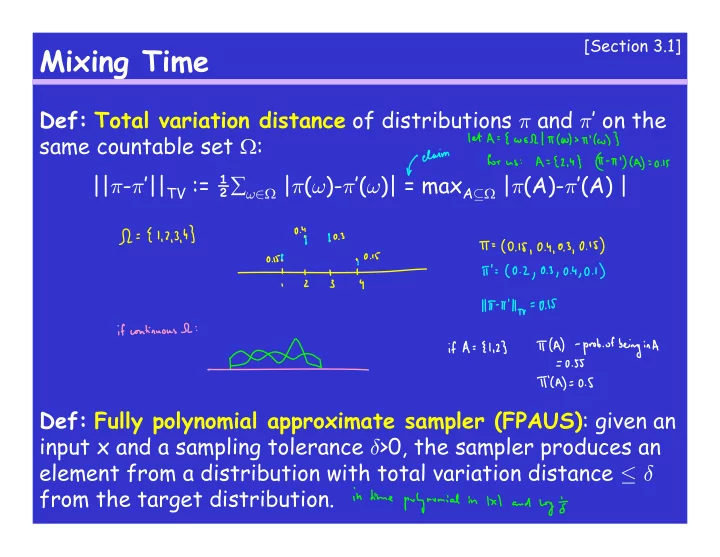
Def: Total variation distance of distributions π and π’ on the same countable set : ||π-π’||TV := ½ω∈ |π(ω)-π’(ω)| = maxA⊆ |π(A)-π’(A) | Def: Fully polynomial approximate sampler (FPAUS): given an input x and a sampling tolerance δ>0, the sampler produces an element from a distribution with total variation distance ≤ δ from the target distribution.

[Section 3.1]

Detailed Balance and Reversibility

Lemma 3.7: Let (,P) be a MC. If distribution π’ on  satisfies π’(x)P(x,y) = π’(y)P(y,x) for every x,y∈, then π’ is a stationary distribution of the MC. Note: the condition from Lemma 3.7 is known as detailed balance (or time reversibility of the MC).

[Section 3.3]

Symmetric MC and the Metropolis Filter

What is the stationary distribution when the MC is symmetric (i.e. P(x,y)=P(y,x) for every x,y) ? Metropolis Filter: Suppose we want a stationary distribution π on  and we have designed the transitions (but not their probabilities) so that the MC is ergodic. How to set up the transition probabilities ?

Mixing Time cont’

Def: Given an ergodic MC (,P) with stationary distribution π, its mixing time from a state x∈ is: τx(²) := min{ t: ||Pt(x,.)-π||TV ≤ ²}. Overall mixing time is τ(²) := maxx∈ τx(²). Note: the definition makes sense, i.e., ||Pt(x,.)-π||TV is a non-increasing function of t. [Lemma 4.2]

[Chapter 4]

Coupling

Recall the MC for colorings:

• Choose a vertex v u.a.r. (uniformly at random)
• Choose a color c u.a.r.
• If none of v’s neighbors is colored by c, recolor v by c.
• Otherwise, keep v’s original color.

We’ll modify the MC to choose a color not used by any of v’s neighbors. Claim: Let q be the number of colors. If q ≥ M+2, where M is the maximum degree in the graph, then MC is ergodic.

[Chapter 4]

Coupling

MC for colorings:

• Choose a vertex v u.a.r. (uniformly at random)
• Choose a color c not used by any neighbor of v u.a.r.
• Recolor v by c.
• Prop. 4.5: Let G be a graph with max.deg. M. Let the number
• f colors q ≥ 2M+1. Then the MC mixes in time:

τ(²) ≤ qn/(q-2M) ln(n/²).

[Chapter 4]

Coupling

Coupling idea:

• Run two identical MC’s.
• They can (and most likely will) be dependent but each

without seeing the other MC follows the prescribed transition probabilities.

• Start the first MC in the stationary distribution, the other

MC starts anywhere.

• Goal: the MC’s coalesce, thus the second MC is also following

the stationary distribution.

• Want to set up the dependence between the MC’s so that

they agree with each other more and more as time progresses.

[Chapter 4]

Coupling

Coupling, formally: Given a MC (,P). A MC on  x is a coupling for the above MC if it goes through states (X0,Y0),(X1,Y1),(X2,Y2),… such that: Pr[Xi+1=x’ | Xi=x, Yi=y] = Pr[Yi+1=y’ | Xi-x, Yi=y] =

[Chapter 4]

Coupling

Warmup: MC on the n-dimensional hypercube (i.e., binary numbers of length n):

• With probability ½ do not do anything.
• Otherwise, choose a random position i and flip the i-th bit.

Coupling:

[Chapter 4]

Coupling

Lemma 4.7 [Coupling Lemma]: Suppose we have a MC with transition matrix P. Let (Xt, Yt) be a coupling of this MC and suppose t:[0,1] N is a fnc such that Pr[Xt(²)  Yt(²) | X0=x, Y0=y] ≤ ². Then, the mixing time of the MC: τ(²) ≤ t(²).

[Chapter 4]

Coupling

Back to colorings – how to couple ?

[Chapter 4]

Coupling

Back to colorings – notation:

[Chapter 4]

Coupling

Back to colorings – notation:

[Chapter 4]

Coupling

Back to colorings – how to couple ?

• What if the colors of v differ ?

[Chapter 4]

Coupling

Back to colorings – how to couple ?

• What if the colors of v agree ?

[Chapter 4]

Coupling

Back to colorings – finishing the argument

[Chapter 4]

Some useful inequalities

Markov’s: If X is a non-negative random variable and a>0, then Pr(X>a) ≤ E(X)/a Chebyshev’s: For any a>0: Pr(|X-E(X)|≥ a) ≤ Var(X)/a2 No name: 1+x ≤ ex

Path Coupling

• simplifies the coupling analysis

Idea:

• define distance between states
• if neighboring states get closer in one step (in expectation),

then all pairs of states get closer in one step

• therefore, we have a coupling

[Chapter 4]

Path Coupling

Applied to colorings:

• distance:
• how to couple neighboring states:

[Chapter 4]

Path Coupling

Now in the math-language (drawing from Lemmas 4.14-6): Lemma: Suppose for every pair of adjacent states X0,Y0: E[distance(X1,Y1) | X0,Y0] ≤ (1-α)distance(X0,Y0) Then, τ(²) ≤ α-1 ln(maxdist/²) where maxdist is the maximum distance between any two states.

[Chapter 4]