
SLIDE 1
- 0.2
0.2 0.4 0.6 0.8 1 1.2
- 0.2
0.2 0.4 0.6 0.8 1 1.2
- 0.2
0.2 0.4 0.6 0.8 1 1.2
- 0.2
0.2 0.4 0.6 0.8 1 1.2
- 0.2
0.2 0.4 0.6 0.8 1 1.2
- 0.2
0.2 0.4 0.6 0.8 1 1.2
- 0.2
0.2 0.4 0.6 0.8 1 1.2
- 0.2
0.2 0.4 0.6 0.8 1 1.2
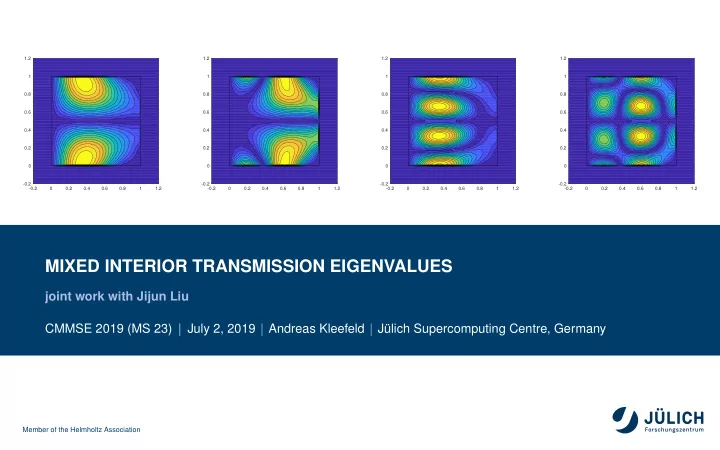
MIXED INTERIOR TRANSMISSION EIGENVALUES
joint work with Jijun Liu CMMSE 2019 (MS 23) | July 2, 2019 Andreas Kleefeld J¨ ulich Supercomputing Centre, Germany
Member of the Helmholtz Association