min ( ). ( , , ). ( , ) l i a i j k V j k i j - - PDF document

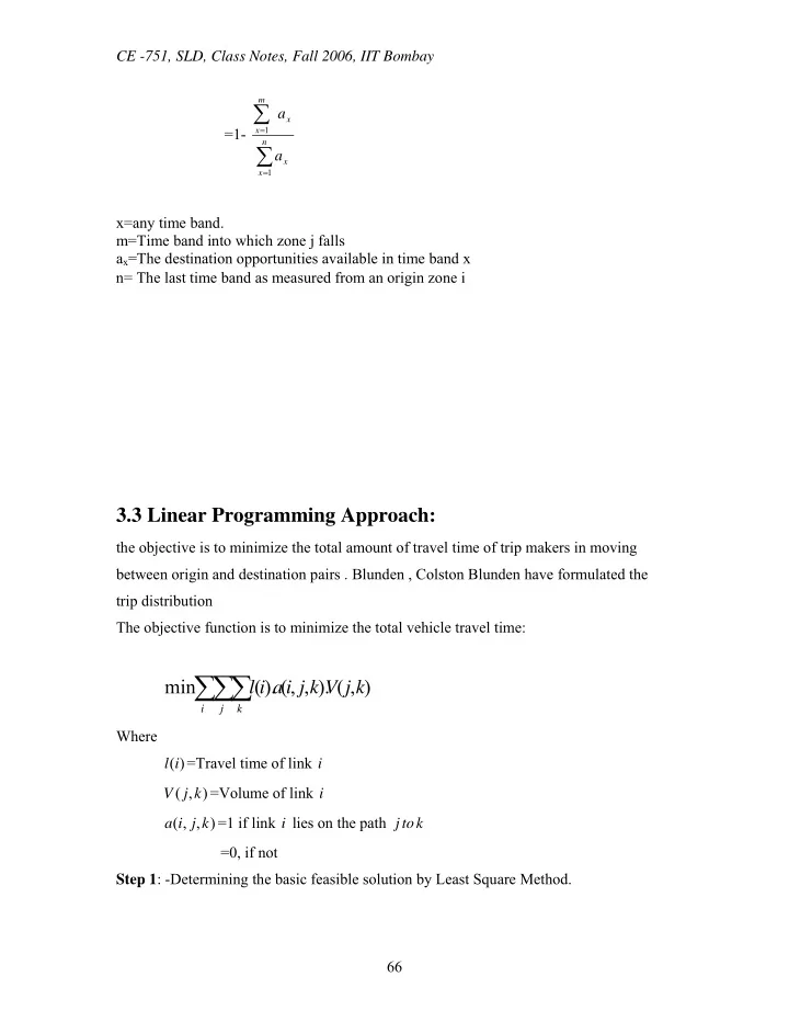
CE -751, SLD, Class Notes, Fall 2006, IIT Bombay 66 =1-

∑ ∑

= = n x x x m x

a a

1 1

x=any time band. m=Time band into which zone j falls ax=The destination opportunities available in time band x n= The last time band as measured from an origin zone i

3.3 Linear Programming Approach:

the objective is to minimize the total amount of travel time of trip makers in moving between origin and destination pairs . Blunden , Colston Blunden have formulated the trip distribution The objective function is to minimize the total vehicle travel time:

∑∑∑

i j k

k j V k j i a i l ) , ( ). , , ( ). ( min

Where ) (i l =Travel time of link i ) , ( k j V =Volume of link i ) , , ( k j i a =1 if link i lies on the path k to j =0, if not Step 1: -Determining the basic feasible solution by Least Square Method.

CE -751, SLD, Class Notes, Fall 2006, IIT Bombay 67 Step 2: -There will be 3+2-1=4 basic variables. Checking for optimality,

• 1. Only simplex method is used to determine the entry variable. If the optimality

condition is satisfied, stop if not go to step 2.

• 2. Determine leaving variable using the simplex feasibility condition.

By the method of multipliers, for each basic variable:

ij j i

c v u = + Letting

3 =

u , I can solve for the remaining as shown in table below

CE -751, SLD, Class Notes, Fall 2006, IIT Bombay 68

3.3.1 Example problem:

Assign the traffic to the various links for the network shown below. E1=4000 E2=5000

• Table. Travel Time Matrix

R5=3000 R2=3000 R3=3000 The objective function is to minimize the total vehicle travel time:

∑∑∑

i j k

k j V k j i a i l ) , ( ). , , ( ). ( min Where ) (i l =Travel time of link i ) , ( k j V =Volume of link i ) , , ( k j i a =1 if link i lies on the path k to j =0, if not subject to constraints 000 , 5 000 , 4 000 , 3 000 , 3 000 , 3

52 42 32 51 41 31 52 51 42 41 32 31

= + + = + + = + = + = + T T T T T T T T T T T T As this is a balanced transportation problem, we can solve in using transportation label

• model. The travel times are in the N-E corner of the each table.

Step 1: -Determining the basic feasible solution by Least Square Method. D O 1 2 3 11 22 4 16 18 5 21 10 3 2 1 4 5

CE -751, SLD, Class Notes, Fall 2006, IIT Bombay 69 1 2 11 22 3 3000 3000 16 18 4 1000 2000 3000 21 10 5 3000 3000 4000 5000

• 1. Cell (3,1) has the least travel time. Assign 3000 to this cell. Row I1 is satisfied,

satisfy column 1.

• 2. Next the cell with the least travel time is (5,2). Assign 3000 to this cell and

adj8ust the total of column 2 to 5000-3000=2000

• 3. Next cell with least travel time is (4,1) and allocate to it 1000
• 4. Allocate 2,000 to cell (4,2)

Step 2: -There will be 3+2-1=4 basic variables. Checking for optimality,

• 3. Only simplex method is used to determine the entry variable. If the optimality

condition is satisfied, stop if not go to step 2.

• 4. Determine leaving variable using the simplex feasibility condition.

By the method of multipliers, for each basic variable:

ij j i

c v u = + Letting

3 =

u , I can solve for the remaining as shown in table below

CE -751, SLD, Class Notes, Fall 2006, IIT Bombay 70 Basic Variable ( ) ,v u Solution (3,1) 11

1 3

= + v u 11

1 =

v (4,1) 16

1 4

= + v u 5

4 =

u (4,2) 18

2 4

= + v u 13

2 =

v 5,2) 10

2 5

= + v u 3

5

− = u I can use the tabulated solutions to get the values of the non-basic variables. Non-basic Variable

ij j i

c v u − + Comment (3,2) 9 22 13

32 2 3

− = − + = − + c v u (5,1) 13 21 11 3

51 1 5

− = − + − = − + c v u The starting solution is

• ptimal

As the problem is minimization, the starting points are the solution as the non-basic variables has non-positive values. The solutions are:

31

T

41

T

42

T

52

T Solution 3000 1000 2000 3000 The assigned trips can shown as: E1=4000 E2=5000 3000 1000 3000 2000 R1=3000 R2=3000 R3=3000 D O 1 2 3 11 22 4 16 18 5 21 10 3 2 1 4 5

CE -751, SLD, Class Notes, Fall 2006, IIT Bombay 71

3.4 Wilson Modified Entropy Model:

The urban and regional scientist faces a number of theoretical problems. His activity is

• ften a multi disciplinary one in the sense that he uses to concepts from several

disciplines- economics, geography, and sociology and so on. The concept of entropy has, until recently, been used primarily in the non social science. It has hoped that ‘entropy’ enables the social scientist to take some of his basic problems in a fruitful way, and thus to make progress which might not be possible so easily which more orthodox tools.

Applications of Entropy:

• 1. It is used for theory building hypothesis (model) development.
• 2. Used in expressing the laws about system dynamics.
• 3. For interpretation procedures for the theories.

The main views of entropy is

• 1. The relationship of entropy to probability and uncertainty.
• 2. The entropy of probability distribution.
• 3. Entropy and Bayesian statistics.

Gravity Model

• Based on land use and transportation network
• Calibrated for many urban areas
• Simple
• Accurate
• Supported by the USDOT

"The number of trips between 2 zones is directly proportional to the number of trip attractions at the destination zone and inversely proportional a function of the travel time"

CE -751, SLD, Class Notes, Fall 2006, IIT Bombay 72 Tij = Trips produced in zone i and attracted to zone j Pi = Trips produced in zone i Aj = Trips attracted in zone j Fij = Friction factor for impedance (usually travel time) between zones i and j Kij = Socioeconomic adjustment factor for trips produced in i and attracted to j How do we determine values for the variables?

• Recall Ps and As come from trip generation
• The sum of productions has to equal the sum of attractions
• Ks are used to force estimates to agree with observed trip interchanges

(careful! do not use too many of these! Have a good reason for using them!)

• Fs are determined by a calibration process (by purpose), and depend upon

the willingness of folks to make trips of certain lengths for certain purposes recall... trip purposes HBW - home based work HBO - home based other NHB - non-home based HBS - home based school

Derivation of Gravity model:

Fij= γ

2 12 2 1

d m m T12=

2 12 2 1

d D O k Double the values of γ, Oi, Dj

CE -751, SLD, Class Notes, Fall 2006, IIT Bombay 73 T12=

2 12 2 1

d D O k Trip end balance is required Balancing factors are Ai & Bj Take the impedance in the form of generalized function £=ln W(Tij) + λi(1)( Oi – ∑

j

Tij) + λj(2)( Di – ∑

i

Tij) + β(C ‐ ∑∑

i j

TijCij) Tij= exp (‐λi(1) ‐λj(2) ‐β(Cij))

∑

j

Tij=Oi or exp (‐λi(1))∑

j

exp (‐λj(2) ‐β(Cij)) exp (‐λi(1))= Oi/Ai ∑

j

exp (‐λj(2) ‐β(Cij))‐1 exp (‐λi(2))= Dj/Bj ∑

j

exp (‐λj(1) ‐β(Cij))‐1 Tij=AiOjBjDJexp(‐βCij) Ai=

i

O

i )

(

1

exp

γ −

Bj=

j

D

ji )

(

2

exp

γ −

Ai= [∑

j j

D exp (‐λj(2) ‐β(Cij))‐1] Bj=[∑

i i

O Ai exp( ‐β(Cij))‐1] Ai= ) exp( 1

∑

−

j ij j

C D B β

CE -751, SLD, Class Notes, Fall 2006, IIT Bombay 74

3.5 Trip Assignment:

3.5.1 All Or Nothing Assignment Model:

All or nothing assignment is basically an extension of finding the minimum paths through a network. It is called all or nothing because every path from origin zone traffic to a destination zone has either all the traffic (if it is assumed as minimum paths) or none of the traffic. The steps followed are:

• 1. Find the minimum path tree from each of the zone centroid nodes to all other

nodes.

• 2. Assign the flow from each origin to each destination node obtained from the trip

table to the arcs comprising the minimum path for that movement.

• 3. Sum the volume on each arc to obtain the total arc volume. If (undirected) link

volume is desired, sum the flows on the two arcs that represent bi-directional link. The All or Nothing Traffic Assignment is illustrated using the following example. 10 11 7 8 7 5 6 10 Home Node Minimum Path tree 11 1 7 1 2 3 4

CE -751, SLD, Class Notes, Fall 2006, IIT Bombay 75 17 2 10 13 7 14 5 3 6 4 8 15 10 Inter node volume, veh/hr is given belo 1 2 3 4 4 3 2 1 ⎥ ⎥ ⎥ ⎥ ⎦ ⎤ ⎢ ⎢ ⎢ ⎢ ⎣ ⎡ − − − − 2050 350 1250 950 1870 650 475 1050 275 350 750 500 275 500 1100 1900 1525 2220 2075 315 LINK 4-3 IS CONGESTED LINK 1 2 3 4

CE -751, SLD, Class Notes, Fall 2006, IIT Bombay 76

3.5.2 Capacity Restrained Method:

This model involves two-travel time versus volume relationships used iteratively to arrive at predictions of volumes on up to four separate routes between any two zones. The first equation utilizes route volume as the dependent variable. The symbolical representation of the graphical portrayal is:

rc r rc r rc r

V L V V d t t ) ( − + =

• -----------------------------------------------------------------(1)

where r t =travel time on route r (minutes)

r

V = Volume of traffic on route r (veh/hr/lane)

rc

V = Critical volume for the route r (veh/hr/lane)

rc

t = unit travel time at the critical volume (min/mile)

r

L = length of the route r (miles) d = delay parameter (min/mile) =0.50 for

r

V <

rc

V =10.0 for

r

V ≥

rc

V The second relationship used for predicting the volume on the route r given travel time: V t t V

m r r r r

∑

=

=

1

/ 1 / 1

• --------------------------------------------------------------------------(2)

where V =the total volume of trips from zone I to j on all routes

r

t =travel time on route r (minutes)

r

V = Volume of traffic on route r (veh/hr/lane) Equation (2) divides up the volume of trips from zone I to j among the various routes in accordance with the reciprocal of the travel times.

CE -751, SLD, Class Notes, Fall 2006, IIT Bombay 77 The steps which are followed will be: i. Find r t from equation (1) ii. Find

r

V by inserting r t in equation (2) iii. Enter the value of

r

V in equation (1) iv. Repeat the same procedure until the changes in volumes or travel times become negligible Example of the TRC Trip Assignment model The interplay between two TRC Trip Assignment equations can be demonstrated through a n example in which a pair of zones is connected by the two routes whose characteristics are shown in table 1 below. Table 1 Example Route Characteristics

Route No.

• No. of

lanes Speed limit (mph) Signals/ mile Length (mile) Critical volume Critical travel time

Travel time with no volume

1 1 30 1 3 600 3 2.5 2 1 50 1 4 1100 2 1.5 Iteration 1: - starts with the ideal travel times for the entire length of each route. Thus, if no traffic were: On route 1, the travel time would equal: 2.5min/mileX3miles = 7.5min On route 2, the travel time would equal: 1.5min/mileX4miles = 6.0min This leads to: lane vph V / 532 ) 1200 ( . 6 / 1 5 . 7 / 1 5 . 7 / 1

1

= + = and lane vph V / 668 ) 1200 ( . 6 / 1 5 . 7 / 1 . 6 / 1

2

= + = From equation (1) taking 5 . = d since both the routes have volumes less than their respective critical volumes, we get:

CE -751, SLD, Class Notes, Fall 2006, IIT Bombay 78 =

1

t 3 600 ) 600 532 ( 50 . . 3 ⎥ ⎦ ⎤ ⎢ ⎣ ⎡ − + = 8.82 min and =

2

t 4 100 , 1 ) 100 , 1 668 ( 50 . . 2 ⎥ ⎦ ⎤ ⎢ ⎣ ⎡ − + = 7.20 min Iteration 2: - lane vph V / 536 ) 1200 ( 72 . 7 / 1 82 . 8 / 1 82 . 8 / 1

1

= + = and lane vph V / 664 ) 1200 ( 72 . 7 / 1 82 . 8 / 1 20 . 7 / 1

2

= + = Then the travel times will be: =

1

t 3 600 ) 600 536 ( 50 . . 3 ⎥ ⎦ ⎤ ⎢ ⎣ ⎡ − + = 8.85min and =

2

t 4 100 , 1 ) 100 , 1 664 ( 50 . . 2 ⎥ ⎦ ⎤ ⎢ ⎣ ⎡ − + = 7.18 min where 5 . = d again since both the routes have volumes less than their respective critical volumes. Since the last set of travel times do not differ significantly from the previous, the procedure can be terminated and hence the final results are: lane vph V / 536

1 =

and lane vph V / 664

2 =

min 85 . 8

1 =

t and

2

t =7.18 lane vph/ The number of iterations is less in this particular case. If the inter zonal volume falls within a range of lane vph/ 300 ±

• f the sum of the critical volumes which in example is

600 + 1,100 = 1,700 lane vph/ . The reason for this is that d parameter will jump from 0.5 to 10.0 and back, causing corresponding fluctuations in the related travel times.

CE -751, SLD, Class Notes, Fall 2006, IIT Bombay 79

3.5.3 Multipath Assignment Model :

McLaughlin developed one of the first multi-path traffic assignment techniques. A driver route selection criteria is used by McLaughlin which is a function of:

• Travel time
• Travel cost
• Accident potential

The minimum resistance paths between each origin and destination pair are calculated with all the link resistances set to values that correspond to a zero traffic volume. The minimum resistance value between an origin and destination pair is increased by 30%. All the paths between the origin and the destination pair with the resistance values less than this maximum value are identified. McLaughlin used certain principles of linear graph theory to accomplish the multi-path

• assignment. Using an electrical analogy it is possible to identify a through variable y that

corresponds to current, or traffic flow. A cross variable x may be identified that corresponds to the potential difference, or traffic pressure. Two postulates from linear graph theory may be introduced that are known as the vertex and circuit postulates. At any vertex

Σ

= e i 1

= aiyi where e = the number of oriented terminal graphs, or elements yi = the through variable of the ith element ai = 0 if the ith element is not connected to v =1 if the ith is oriented away from V =-1 if the ith element is oriented toward For any circuit,

1

=

Σ

=

bixi

e i

CE -751, SLD, Class Notes, Fall 2006, IIT Bombay 80 where e = the number of oriented terminal graphs, or elements xi = the cross variable of the ith element bi = 0 if the ith element is not in the jth circuit =1 if the ith element orientation is the same as the jth circuit =-1 if the ith element orientation is opposite to the jth circuit A sub-graph is then established for each origin and destination pair with these representing two vertices. The connecting elements are the acceptable paths between the vertices plus one flow driver element that corresponds to the car travel demand between the origin and destination pair. The travel demand is assigned among the potential paths building phase. The traffic assigned to each alternative path must be such that the alternative paths have an equal across variable value. The cross variable X , the resistance value ) (y R and the through variable y for each path are assumed to be related as follows: y y R X ) ( = The above equation is analogous to Ohm’s Law in that the potential is equal to the resistance times the flow. In this case the resistance along a path is assumed to be a function of the flow along that path The figure 1 below represents the way McLaughlin illustrated the assignment method. A schematic two-way street system is shown along with the link descriptions and then trip

• table. The minimum path trees were determined for all origin-destination pairs using the

resistance function for the zero flow, and these are given in table 1 below. Multiplied the minimum path resistance values and the paths whose resistance values were less than this higher value were determined and these paths are also given in table 2 below. The trip table inputs were assigned directly for the origin-destination pairs with only one

• path. Sub-graphs were formed for the remaining trip table inputs and solved by the chord

CE -751, SLD, Class Notes, Fall 2006, IIT Bombay 81 formulation of linear graph theory. Figure 2 shows the sub-graph for the origin1 and destination 3. The circuit equations may be represented in the general form as: ⎥ ⎥ ⎥ ⎥ ⎥ ⎦ ⎤ ⎢ ⎢ ⎢ ⎢ ⎢ ⎣ ⎡ u B B u B B

22 21 12 11

⎥ ⎥ ⎥ ⎥ ⎦ ⎤ ⎢ ⎢ ⎢ ⎢ ⎣ ⎡

− − − − 2 2 1 c i c b b

X X X X where

11

B … =coefficient matrices corresponding to the branches u =a unit matrix corresponding to the chords

1 − b

X …=the column matrices of the branches

1 − c

X ..= the column matrices of the chords 1 2 3 4

CE -751, SLD, Class Notes, Fall 2006, IIT Bombay 82 Link Characteristics No. Link Length (miles) Maximum Capacity (veh/hr) Free speed (mph) 1 1-2 1.0 1200 40 2 1-4 2.0 4000 50 3 2-1 1.0 1200 40 4 2-3 0.5 1000 30 5 3-2 0.5 1000 30 6 3-4 0.5 1000 30 7 4-1 2.0 4000 50 8 4-3 0.5 1000 30 Trip Table Destination Origin 1 2 3 4 1 100 100 2500 2 300* 100 800 Fig 1. Multi-path assignment example problem Table 1 Paths for multi-path example Origin Destination Minimum path* Diversion path* Minimum τ Path Diversion τ Path 2 1,2

• 1,2
• 3

1,2,3 1,4,3 1,2,3

• 1

4 1,4

• 1,4

1,2,3,4 1 2,1

• 2,1
• 3

2,3

• 2,3
• 2

4 2,3,4

• 2,3,4

CE -751, SLD, Class Notes, Fall 2006, IIT Bombay 83 * Based on the resistance function = ) ( ) ( p t p s τ based on the resistance function = ) ( p S Where ) (p s = travel cost (operating, accident, and comfort) as a function of the volume -to-capacity ratio p = ) ( p t Travel time as a function of the volume-to-capacity ratio p = ) ( p S Travel cost (operating, accident, comfort, and time) as a function of the volume -to-capacity ratio p 3 1 1 3 2 Branch Element 1- path 1,2,3 Chords 2- path 1,4,3 3-trip table input Fig 2.Subgraph of the origin 1 and destination 2 The first term is non-existent in this system and the circuit equations are: ⎥ ⎥ ⎥ ⎦ ⎤ ⎢ ⎢ ⎢ ⎣ ⎡ u B u B

22 12

⎥ ⎥ ⎥ ⎦ ⎤ ⎢ ⎢ ⎢ ⎣ ⎡

− − − 2 1 2 c c b

X X X =0 The terminal equations of the street components may be represented by:

CE -751, SLD, Class Notes, Fall 2006, IIT Bombay 84 ⎥ ⎥ ⎥ ⎦ ⎤ ⎢ ⎢ ⎢ ⎣ ⎡

− − 1 2 c b

X X = ⎥ ⎥ ⎥ ⎦ ⎤ ⎢ ⎢ ⎢ ⎣ ⎡

− − 1 2 c b

R R ⎥ ⎥ ⎥ ⎦ ⎤ ⎢ ⎢ ⎢ ⎣ ⎡

− − 1 2 c b

Y Y Where

2 − b

R = the sum of the link resistances corresponding to branch paths

1 − c

R =The sum of the link resistances corresponding to chord paths

2 − b

Y =The flow on the branch path

1 − c

Y =Flow on the chord paths For the demand assignment: ⎥ ⎥ ⎥ ⎦ ⎤ ⎢ ⎢ ⎢ ⎣ ⎡

2 1

X X = ⎥ ⎥ ⎥ ⎦ ⎤ ⎢ ⎢ ⎢ ⎣ ⎡ 17 . 12 51 . 9 ⎥ ⎥ ⎥ ⎦ ⎤ ⎢ ⎢ ⎢ ⎣ ⎡

2 1

Y Y The sub-graph fundamental circuit equations are then substituted into the chord set of equations ⎥ ⎥ ⎥ ⎦ ⎤ ⎢ ⎢ ⎢ ⎣ ⎡ u

2 − c

X + ⎥ ⎥ ⎥ ⎦ ⎤ ⎢ ⎢ ⎢ ⎣ ⎡

22 12

B u B ⎥ ⎥ ⎥ ⎦ ⎤ ⎢ ⎢ ⎢ ⎣ ⎡

− − 1 2 c b

R R ⎥ ⎥ ⎥ ⎦ ⎤ ⎢ ⎢ ⎢ ⎣ ⎡

22 12

u B B

T T

⎥ ⎥ ⎥ ⎦ ⎤ ⎢ ⎢ ⎢ ⎣ ⎡

− − 2 1 c c

Y Y =0 Where

12

B =a column matrix with coefficients equal to -1; the number of rows in this matrix correspond to the number of non driver chords in the sub-graph; or it corresponds to the number of paths less 1 between an origin-destination pair

22

B =+1, corresponding to the driver or trip table input

1 − c

Y =The unknown flows for the non driver chord elements

2 − c

Y =The through driver, or trip table input

CE -751, SLD, Class Notes, Fall 2006, IIT Bombay 85 The specific formulation for this example is: ⎥ ⎥ ⎥ ⎦ ⎤ ⎢ ⎢ ⎢ ⎣ ⎡ 1

3

X + ⎥ ⎥ ⎥ ⎦ ⎤ ⎢ ⎢ ⎢ ⎣ ⎡− 1 1 1 1 ⎥ ⎥ ⎥ ⎦ ⎤ ⎢ ⎢ ⎢ ⎣ ⎡ 17 . 12 51 . 9 ⎥ ⎥ ⎥ ⎦ ⎤ ⎢ ⎢ ⎢ ⎣ ⎡− 1 1 1 ⎥ ⎥ ⎥ ⎦ ⎤ ⎢ ⎢ ⎢ ⎣ ⎡ 100

2

Y =0 Taking the first set of the above equations, the solution is

2

Y =44 vehicles per hour, and the flow on element 1 is solved by subtraction;

1

Y =100-44=56veh/hr. The results of the demand assignment are presented in table 2 Table 2 Link volumes for multi-path example No. Link R

1

Y

1

R

2

y

3

y

4

y 1 12 4.90 156 4.98 138 1,290 625 2 14 7.56 2,544 8.42 2,562 1,410 2,075 3 21 4.90 300 5.00 300 300 300 4 23 4.61 956 16.40 938 2,090 1,425 5 32 4.61 4.61 6 34 4.61 800 5.80 1,890 1,890 1,225 7 41 7.56 7.56 8 43 4.61 44 4.61 62 In McLaughlin’s assignment procedure, new link and path resistance values are calculated for the capacity restraint assignment that corresponds to the flows obtained from the demand assignment. The procedure described above is employed again to calculate the restrained volumes. If these volumes are within tolerable limits of the demand volume then the restraint assignment is complete, otherwise an iterative is required. An iterative solution is achieved by averaging the link volumes according to the following expression: Y = n yi

n i 1 =

Σ ]

CE -751, SLD, Class Notes, Fall 2006, IIT Bombay 86 Where Y = the average assigned volumes

i

Y =The trips assigned to the links during the ith iteration of the linear graph procedure including iterations n= the number of linear graph iterations Burrell has proposed a technique for generating multiple paths through a traffic network. This method assumes that the user does not know the actual travel times on the links but associates a supposed travel time on each link that is drawn at random from a distribution

• f times. It assumes that the user finds and uses a route that minimizes the sum of the

supposed link times. Burrell assumes that a group of trips originating from a particular zone have the same set

• f supposed link times and consequently there is only one tree for each zone of
• production. A rectangular distribution that could assume eight separate magnitudes was

assumed and the ranges of distributions for each of the links were selected so that the ratio of the mean absolute deviation to actual link time was the same for all links. The demand or capacity restrained assignments are then made to the paths selected in the above manner. Another multi-path assignment technique has been proposed by Dial. With this technique each potential path between a particular origin and destination pair is assigned a probability of use that then allows the path flows to be estimated.

CE -751, SLD, Class Notes, Fall 2006, IIT Bombay 87

3.6 GRAPH THEORY APPROACH

Graph theory is basically a branch of topology. Geometric structure of a transport network, which is the topological pattern formed by nodes and routes is studied by graph

• theory. The use of graph theoretic approach in road network analysis is to compare and

evaluate one network analysis with the other which may be in the same region or in different regions. It can be also used to check connectivity and accessibility level of different nodes. Connectivity: Its concept involves following terms: 1. Degree of vertex: Number of edges meeting at the vertex. 2. Path: Collection of vertices and a subset of their incident edges so that degree

• f each internal vertex is two or more and the degree of each terminal vertex

is one. 3. Circuits: Closed path where all vertices are of degree two or more. 4. Connected and Unconnected Graph: Connected if there exist at least one path between any pair of vertices in graph. In unconnected, there are pairs of points or vertices which cannot be joined by a path. Structural and geometrical properties of alternative transport networks can be measured in terms of following graph theoretic measures: 1. Beta Index: Ratio of total number of links to the total number of nodes in network. Mathematically: β = (e/v) Where: e and v are, respectively, number of edges and vertices in network. 2. Cyclomatic Number: A count of the number of fundamental circuits existing in the graph. It is an measure of redundancy in the system. Mathematically: μ = e – (v – p) Where: p is number of maximal connected sub graph. 3. Gamma Index: Ratio of the observed number of edges in network to maximum number of edges which may exist between specified number of vertices.

CE -751, SLD, Class Notes, Fall 2006, IIT Bombay 88 Mathematically: γ = e x 100/ (3(v – 2) 4. Alpha Index: Ratio of the observed number of fundamental circuits to the maximum possible number of complete circuits. Mathematically: α = μ x 100/(2v – 5) 5. Associate Number: The number of links needed to connect a node to the most distant node from it. The node which has low associate number is most accessible. 6. Shimbel Index: Measure of accessibility which indicates the number of links needed to connect any node with all other nodes in the network by the shortest

• path. The node having lower shimbel index is the most accessible.

7. Dispersion Index: It is the measure of connectivity of transport network and

• btained by sum of the shimbel index.

Mathematically,

∑ ∑

= =

=

v i ij v j

d DI

1 1

8. Degree of Connectivity: Ratio of maximum possible number of routes to have Complete connectivity to observed number of routes in network. Degree of Connectivity = ((v(v – 1)/2)/e

Example 1:

The solution for the problem can be done in tabular form as follows: A B C D E F G