Midterm 2 Review and Minimum Spanning Trees Tyler Moore CSE 3353, - - PDF document

Midterm 2 Review and Minimum Spanning Trees

Tyler Moore

CSE 3353, SMU, Dallas, TX

March 28, 2013

Portions of these slides have been adapted from the slides written by Prof. Steven Skiena at SUNY Stony Brook, author

• f Algorithm Design Manual. For more information see http://www.cs.sunysb.edu/~skiena/

Administrivia

Midterm 2 next Tuesday, April 2

Covers Graph Algorithms and Recurrence Relations All material through Tuesday March 26 (including Kosaraju’s SCC algorithm, two vertex coloring algorithm, but NOT weighted algorithms) You are allowed notes on one side of a 3x5 index card Review today I will be traveling at a conference next week, so no normal office hours Come see me with any questions this week (extra office hours today 4-5pm and this Friday 1-2pm)

Next Fall I’m teaching CSE 5338 Security Economics

T/Th 11am-12:20pm Counts as upper-division CS elective, also can be taken as 7338 for 4+1 students and applied to M.S. in Security Engineering Learn to apply microeconomics and data analytics to security problems No security or economics background required Course webpage: http://lyle.smu.edu/~tylerm/courses/econsec/

2 / 37

HW2 review: Q1d and Q1e

There are several data structures you can use to represent a graph’s structure when doing traversal

We primarily studied dictionaries mapping a node to its children To identify paths, it is better to use a dictionary mapping a node to its parents

3 / 37

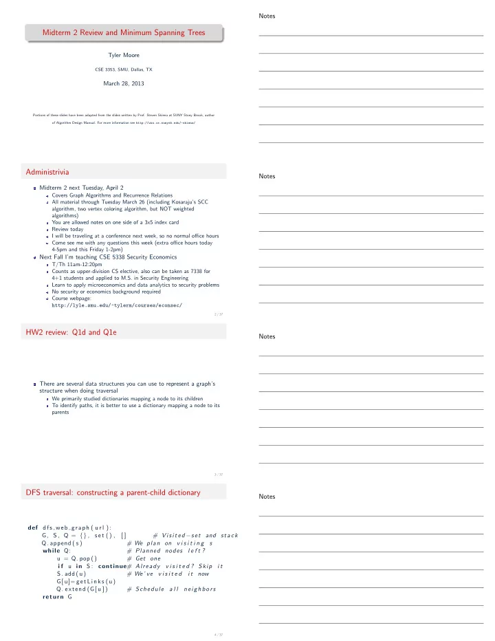
DFS traversal: constructing a parent-child dictionary

def dfs web graph ( u r l ) : G, S , Q = {} , s e t () , [ ] # V i s i t e d −s e t and stack

• Q. append ( s )

# We plan on v i s i t i n g s while Q: # Planned nodes l e f t ? u = Q. pop () # Get one i f u in S : continue# Already v i s i t e d ? Skip i t S . add (u) # We ’ ve v i s i t e d i t now G[ u]= getLinks (u)

• Q. extend (G[ u ] )

# Schedule a l l neighbors return G

4 / 37

Notes Notes Notes Notes

DFS traversal: constructing a child-parent dictionary

def dfs web parent s ( u r l ) : P, Q = { u r l : None } , [ u r l ]# Parents and FIFO queue while Q: u = Q. pop () # Constant−time f o r deque for v in getLinks (u ) : i f v in P: continue # Already has parent P[ v ] = u # Reached from u : u i s parent

• Q. append ( v )

return P

5 / 37

Q1d: Find shortest path between 2 URLs

def f i n d s h o r t e s t p a t h ( url1 , u r l 2 ) : #s t a r t with a BFS t r a v e r s a l to

• btain

c hild −parent mapping P = bfs web parent s ( u r l 1 ) u = u r l 2 #make sure the URL e x i s t s i f u r l 2 not in P: return ”No path between URLs e x i s t s ” #b u i l d the path in r e v e r s e from the d e s t i n a t i o n u r l 2 path = [ u ] while P[ u ] != u r l 1 : i f P[ u ] i s None : #g i v e up i f we f i n d the root return ”No path between URLs e x i s t s ” path . append (P[ u ] ) u = P[ u ] path . append ( u r l 1 ) #don ’ t f o r g e t to add the source path . r e v e r s e () #r e o r d e r the path to s t a r t from u r l 1 return path

6 / 37

Q1d: Find longest shortest path for a URL

def find max depth ( u r l ) : P = bfs web parent s ( u r l ) maxpath =[] #keep track

• f

the l o n g e s t path seen so f a r for us in P. keys ( ) : #check a l l URLs re achable from u r l u = us path = [ u ] #b u i l d a path from us to u r l while P[ u ] i s not None : #loop t i l we f i n d the root path . append (P[ u ] ) u = P[ u ] i f l e n ( path)> l e n ( maxpath ) : #i s the new path l o n g e r than c u r r e n t max? path . r e v e r s e () #r e v e r s e

• ur new m a x l i s t

maxpath = l i s t ( path ) #r e p l a c e maxpath return maxpath

7 / 37

Coding expectations for the Midterm

You should be able to understand written code You should be prepared to write a small amount of code Note: you will not be asked to write any code that is directly lifted from the slides, so please don’t fill up your notecard with all the code you’ve seen on slides Let’s go through one example question

8 / 37

Notes Notes Notes Notes

Strongly connected components

A strongly connected component is the maximal subset of a graph with a directed path between any two vertices A B C a b c d e f g h i

9 / 37

Strongly connected components

A B C a b c d e f g h i A B C Are supernodes in a DAG?

10 / 37

Strongly connected components

What if we transpose all edges? A B C a b c d e f g h i SCCs don’t change A B C Supernodes still in DAG

10 / 37

Kosaraju’s algorithm for finding SCCs

1 Get a topological sort of all vertices 2 Transpose the graph (reverse all edges) 3 Traverse the graph in topologically sorted order, adding an SCC each

time a dead end is reached.

11 / 37

Notes Notes Notes Notes

Kosaraju’s Algorithm for Finding Strongly Connected Components

• 1. Get a topological sort of all vertices

a b c d e f g h i topsort: [a, b, e, f, g, c, d, h, i] seen: {} sccs: []

12 / 37

Kosaraju’s Algorithm for Finding Strongly Connected Components

• 2. Reverse all edges

a b c d e f g h i topsort: [a, b, e, f, g, c, d, h, i] seen: {} sccs: []

12 / 37

Kosaraju’s Algorithm for Finding Strongly Connected Components

• 3. Traverse the graph in topologically sorted order, adding an SCC each

time a dead end is reached. 1st SCC a b c d e f g h i topsort: [a, b, e, f, g, c, d, h, i] seen: {a,b,c,d} sccs: [{a,b,c,d}]

12 / 37

Kosaraju’s Algorithm for Finding Strongly Connected Components

• 3. Traverse the graph in topologically sorted order, adding an SCC each

time a dead end is reached. 1st SCC 2nd SCC a b c d e f g h i topsort: [a, b, e, f, g, c, d, h, i] seen: {a,b,c,d,e,g,f} sccs: [{a,b,c,d},{e,g,f}]

12 / 37

Notes Notes Notes Notes

Kosaraju’s Algorithm for Finding Strongly Connected Components

• 3. Traverse the graph in topologically sorted order, adding an SCC each

time a dead end is reached. 1st SCC 2nd SCC 3rd SCC a b c d e f g h i topsort: [a, b, e, f, g, c, d, h, i] seen: {a,b,c,d,e,g,f,h,i} sccs: [{a,b,c,d},{e,g,f},{h,i}]

12 / 37

Code for Kosaraju’s SCC Algorithm

def t r (G) : # Transpose ( rev . edges

• f ) G

GT = {} for u in G: GT[ u ] = s e t () # Get a l l the nodes in there for u in G: for v in G[ u ] : GT[ v ] . add (u) # Add a l l r e v e r s e edges return GT def scc (G) : GT = t r (G) # Get the transposed graph sccs , seen = [ ] , s e t () for u in d f s t o p s o r t (G) : # DFS s t a r t i n g p o i n t s i f u in seen : continue # Ignore covered nodes C = walk (GT, u , seen ) # Don ’ t go ”backward” ( seen ) seen . update (C) # We ’ ve now seen C sccs . append (C) # Another SCC found print sccs

13 / 37

Exercise: Apply Kosaraju’s SCC Algorithm

Graph G a d g b e h c f i Transpose(G) a d g b e h c f i What is the topological sort of G? Let’s make the DFS tree What are the strongly connected components?

14 / 37

Vertex-coloring problem

15 / 37

Notes Notes Notes Notes

Vertex-coloring problem

The vertex-coloring problem seeks to assign a label (aka color) to each vertex of a graph such that no edge links any two vertices of the same color Trivial solution: assign each vertex a different color However, goal is usually to use as few colors as possible Next Thursday, Prof. Matula will give a guest lecture where he proves that any planar graph can be colored by at most 4 distinct colors.

16 / 37

Applications of the vertex-coloring problem

Apart from working at National Geographic, when might you encounter a vertex-coloring problem? Vertex-coloring problems arise in scheduling problems, where access to shared resources must be coordinated Example: register allocation by compilers

Variables are used for fixed timespan (after initialization, before final use) Two variables with intersecting lifespans can’t be put in the same register We can build a graph with variables assigned to vertices and edges drawn between vertices if the variables’ lifespan intersects Color the graph, and assign variables to the same register if their vertices have the same color

17 / 37

Vertex-coloring problem special case: two colors

A bipartite graph is a graph whose vertices can be divided into disjoint sets U and V such that every edge connects a vertex in U to one in V . Bipartite graphs arise in matching problems: matching workers to jobs, matching kidney donors with recipients, finding heterosexual mates If we can color a graph’s vertices using just two colors, then we have a bipartite graph Problem: given a graph, find its two-coloring or report that a two-coloring is not possible U V

18 / 37

Two-coloring algorithm

1 Suppose there are two colors: blue and red. 2 Color the first vertex blue. 3 Do a breadth-first traversal. For each newly-discovered node, color it

the opposite of the parent (i.e., red if parent is blue)

4 If the child node has already been discovered, check if the colors are

the same as the parent. If so, then the graph isn’t bipartite.

5 If the traversal completes without any conflicting colors, then the

graph is bipartite.

19 / 37

Notes Notes Notes Notes

Two-coloring algorithm example 1

Undirected Graph a b c d e f g Breadth-First Search Tree a b c d e f g

1 2 3 4 6 9 5 7

20 / 37

Two-coloring algorithm example 2

Undirected Graph a b c d e f g

CONFLICT

Breadth-First Search Tree a b c d e f g

1 2 3 4 6 9 5 7 8

21 / 37

Recurrence Relations

Recurrence relations specify the cost of executing recursive functions. Consider mergesort

1

Linear-time cost to divide the lists

2

Two recursive calls are made, each given half the original input

3

Linear-time cost to merge the resulting lists together

Recurrence: T(n) = 2T( n

2) + Θ(n)

Great, but how does this help us estimate the running time?

22 / 37

Enter the Master Theorem!

Definition

The Master Theorem For any recurrence relation of the form T(n) = aT(n/b) + c · nk , T(1) = c, the following relationships hold: T(n) =      Θ(nlogb a) if a > bk Θ(nk log n) if a = bk Θ(nk) if a < bk. So what’s the complexity of Mergesort? Mergesort recurrence: T(n) = 2T( n

2) + Θ(n)

Since a = 2, b = 2, k = 1, 2 = 21. Thus T(n) = Θ(nk log n)

23 / 37

Notes Notes Notes Notes

Apply the Master Theorem

Definition

The Master Theorem For any recurrence relation of the form T(n) = aT(n/b) + c · nk , T(1) = c, the following relationships hold: T(n) =      Θ(nlogb a) if a > bk Θ(nk log n) if a = bk Θ(nk) if a < bk. Let’s try another one: T(n) = 3T( n

5) + 8n2

Well a = 3, b = 5, c = 8, k = 2, and 3 < 52. Thus T(n) = Θ(n2)

24 / 37

Apply the Master Theorem

Definition

The Master Theorem For any recurrence relation of the form T(n) = aT(n/b) + c · nk , T(1) = c, the following relationships hold: T(n) =      Θ(nlogb a) if a > bk Θ(nk log n) if a = bk Θ(nk) if a < bk. Now it’s your turn: T(n) = 4T( n

2) + 5n

25 / 37

What’s going on in the three cases?

Definition

The Master Theorem For any recurrence relation of the form T(n) = aT(n/b) + c · nk , T(1) = c, the following relationships hold: T(n) =      Θ(nlogb a) if a > bk Θ(nk log n) if a = bk Θ(nk) if a < bk.

1 Too many leaves: leaf nodes outweighs sum of divide and glue costs 2 Equal work per level: split between leaves matches divide and glue

costs

3 Too expensive a root: divide and glue costs dominate 26 / 37

Weighted graph algorithms (material from here on will NOT be on midterm

In the graphs we’ve studied so far, all edges are treated the same For many applications, this representation does not make sense For example, road networks have capacity, distance, speed limits Beyond DFS/BFS exists an alternate universe of algorithms for edge-weighted graphs Algorithms that take into account edge weights are inevitably more complicated than those for unweighted graphs, but can be used in many more applications.

27 / 37

Notes Notes Notes Notes

Weighted Graph Data Structures

a b d c e f h g

2 1 3 9 4 4 3 8 7 5 2 2 2 1 6 9 8

Nested Adjacency Dictionaries w/ Edge Weights

N = { ’ a ’ :{ ’ b ’ : 2 , ’ c ’ : 1 , ’ d ’ : 3 , ’ e ’ : 9 , ’ f ’ :4 } , ’ b ’ :{ ’ c ’ : 4 , ’ e ’ :3 } , ’ c ’ : { ’ d ’ : 8} , ’ d ’ :{ ’ e ’ : 7} , ’ e ’ : { ’ f ’ : 5} , ’ f ’ :{ ’ c ’ : 2 , ’ g ’ : 2 , ’ h ’ : 2} , ’ g ’ : { ’ f ’ : 1 , ’ h ’ :6 } , ’ h ’ :{ ’ f ’ : 9 , ’ g ’ :8} } > > > ’ b ’ i n N[ ’ a ’ ] # Neighborhood membership True > > > l e n (N[ ’ f ’ ] ) # Degree 3 > > > N[ ’ a ’ ] [ ’ b ’ ] # Edge weight f o r ( a , b ) 2

28 / 37

Minimum Spanning Trees

A tree is a connected graph with no cycles A spanning tree is a subgraph of G which has the same set of vertices

• f G and is a tree

A minimum spanning tree of a weighted graph G is the spanning tree

• f G whose edges sum to minimum weight

There can be more than one minimum spanning tree in a graph (consider a graph with identical weight edges) Minimum spanning trees are useful in constructing networks, by describing the way to connect a set of sites using the smallest total amount of wire

29 / 37

Minimum Spanning Trees

30 / 37

Why Minimum Spanning Trees

The minimum spanning tree problem has a long history – the first algorithm dates back to at least 1926! Minimum spanning trees are taught in algorithms courses since

1

it arises in many applications

2

it gives an example where greedy algorithms always give the best answer

3

Clever data structures are necessary to make it work efficiently

In greedy algorithms, we decide what to do next by selecting the best local option from all available choices, without regard to the global structure.

31 / 37

Notes Notes Notes Notes

Prim’s Algoirhtm

If G is connected, every vertex will appear in the minimum spanning

• tree. (If not, we can talk about a minimum spanning forest.)

Prims algorithm starts from one vertex and grows the rest of the tree an edge at a time. As a greedy algorithm, which edge should we pick? The cheapest edge with which can grow the tree by one vertex without creating a cycle.

32 / 37

Prim’s Algorithm

During execution each vertex v is either in the tree, fringe (meaning there exists an edge from a tree vertex to v) or unseen (meaning v is more than one edge away). def Prim-MST(G): Select an arbitrary vertex s to start the tree from. While (there are still non-tree vertices) Select the edge of minimum weight between a tree and nontree vertex. Add the selected edge and vertex to the minimum spanning tree.

33 / 37

Example Run of Prim’s Algorithm

a b c d e f g

7 8 5 9 7 5 15 6 8 9 11

d a f b e c g

34 / 37

Prim’s Algorithm

a b c d e f g

7 8 5 9 7 5 15 6 8 9 11

d a f b e c g

G = { ’ a ’ : { ’ b ’ : 7 , ’ d ’ :5 } , ’ b ’ : { ’ a ’ : 7 , ’ d ’ : 9 , ’ c ’ : 8} , ’ c ’ : { ’ b ’ : 8 , ’ e ’ : 5} , ’ d ’ : { ’ a ’ : 5 , ’ b ’ : 9 , ’ e ’ : 15 , ’ f ’ : 6} , ’ e ’ : { ’ b ’ : 7 , ’ c ’ : 5 , ’ d ’ : 15 , ’ f ’ : 8 , ’ g ’ : 9} , ’ f ’ : { ’ d ’ : 6 , ’ e ’ : 8 , ’ g ’ :11} , ’ g ’ : { ’ e ’ : 9 , ’ f ’ :11} }

35 / 37

Notes Notes Notes Notes

Prim’s Algorithm Implementation

from heapq import heappop , heappush def prim mst (G, s ) : V, T = [ ] , { } # V: v e r t i c e s i n MST, T: MST # P r i o r i t y Queue ( weight , edge1 , edge2 ) Q = [ ( 0 , None , s ) ] while Q: , p , u = heappop (Q)#choose edge w/ s m a l l e s t weight i f u i n V: continue #s k i p any v e r t i c e s a l r e a d y i n MST

• V. append ( u )

#b u i l d MST s t r u c t u r e i f p i s None : pass e l i f p i n T: T[ p ] . append ( u ) e l s e : T[ p ]=[ u ] f o r v , w i n G[ u ] . items ( ) : #add new edges to f r i n g e heappush (Q, (w, u , v ) ) return T ””” > > > prim mst (G, ’ d ’) { ’ a ’ : [ ’ b ’ ] , ’ c ’ : [ ’ e ’ ] , ’ b ’ : [ ’ c ’ ] , ’ e ’ : [ ’ g ’ ] , ’ d ’ : [ ’ a ’ , ’ f ’ ] }

36 / 37

Output from Prim’s Algorithm Implementation

a b c d e f g

7 8 5 9 7 5 15 6 8 9 11

d a f b e c g

>>> prim_mst(G,’d’) {’a’: [’b’], ’c’: [’e’], ’b’: [’c’], ’e’: [’g’], ’d’: [’a’, ’f’]}

37 / 37

Notes Notes Notes Notes