METHODS OF REGULARIZATION AND THEIR JUSTIFICATIONS WON (RYAN) LEE - PDF document

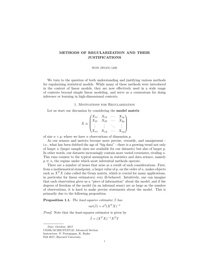
METHODS OF REGULARIZATION AND THEIR JUSTIFICATIONS WON (RYAN) LEE We turn to the question of both understanding and justifying various methods for regularizing statistical models. While many of these methods were introduced in the context of linear models, they are now effectively used in a wide range of contexts beyond simple linear modeling, and serve as a cornerstone for doing inference or learning in high-dimensional contexts. 1. Motivations for Regularization Let us start our discussion by considering the model matrix  X 11 X 12 · · · X 1 p  X 21 X 22 · · · X 2 p   X ≡  . . .  ... . . .   . . .   X n 1 X n 2 · · · X np of size n × p , where we have n observations of dimension p . As our sensors and metrics become more precise, versatile, and omnipresent - i.e., what has been dubbed the age of “big data” - there is a growing trend not only of larger n (larger sample sizes are available for our datasets) but also of larger p . In other words, our datasets increasingly contain more varied covariates, rivaling n . This runs counter to the typical assumption in statistics and data science, namely p ≪ n , the regime under which most inferential methods operate. There are a number of issues that arise as a result of such considerations. First, from a mathematical standpoint, a larger value of p , on the order of n , makes objects such as X T X (also called the Gram matrix, which is crucial for many applications, in particular for linear estimators) very ill-behaved. Intuitively, one can imagine that each observation gives us a “piece of information” about the model, and if the degrees of freedom of the model (in an informal sense) are as large as the number of observations, it is hard to make precise statements about the model. This is primarily due to the following proposition. Proposition 1.1. The least-squares estimator ˆ β has β ) = σ 2 ( X T X ) − 1 var (ˆ Proof. Note that the least-squares estimator is given by β = ( X T X ) − 1 X T Y ˆ Date : October, 2017 CS109/AC209/STAT121 Advanced Section Instructors: P. Protopapas, K. Rader Fall 2017, Harvard University. 1

2 WON (RYAN) LEE Thus, the variance can be computed as β ) = ( X T X ) − 1 X T var( Y )[( X T X ) − 1 X T ] T = σ 2 ( X T X ) − 1 var(ˆ as desired, noting that var( Y ) = σ 2 I . � Thus, an unstable ( X T X ) − 1 implies the instability of the variance of our esti- mator. In other words, small changes in our data can yield large changes for the variability of the estimator, which is problematic. Second, from scientist’s point of view, it is an extremely unsatisfying situation for a statistical analysis to yield a conclusion such as Y = α 1 X 1 + α 2 X 2 + · · · + α 5000 X 5000 Regardless of how complicated the system or experiment may be, it is impossible for the human mind to be able to interpret the effect of thousands of predictors. Indeed, psychologists have found that human beings can typically only hold seven items in memory at once (though later studies argue for even fewer). Consequently, it is desirable to be able to derive a smaller model despite the existence of many predictors - a task that is related to regularization but is known as variable se- lection . In general, model parsimony is a goal often sought after in statistical methodology, as it helps shed light on the relationship between the predictors and response variables. Third, from a statistician’s or machine learner’s viewpoint, it is troubling to have as many predictors as there are observations, which is related to the mathematical problem named above. For example, suppose that n = p , and we are considering a linear model Y = Xβ + ǫ Then, if X is full-rank, we can simply invert the matrix to obtain β = X − 1 Y , which will yield perfect results on the linear regression task. However, the model has learned nothing , so has dramatically failed at the implicit task at hand. This can be seen by the fact that such a model, which is said to be overfit , will typically have no generalization properties; that is, on unseen data, it will generally perform very poorly. This is evidently an undesirable scenario. Thus, we are drawn to methods of regularization , which combat such tenden- cies by (usually) putting constraints on the magnitude of the coefficients β . This prevents the scenario from the above paragraph; if we constrain β sufficiently, it will not be able to take the perfect precision value β = X − 1 Y , and thus will (hopefully) be led to a value in which learning happens. 2. Deriving the Ridge Estimator The ridge estimator was proposed as an ad hoc fix to the above instability issues by Hoerl and Kennard (1970). 1 From this point onward, we will generally assume that the model matrix is standardized, with column means set to zero and sample variances set to one. One of the signs that the matrix ( X T X ) − 1 may be unstable (or super-collinear ) is if the eigenvalues of the X T X are close to zero. This is because by the spectral decomposition, X T X = Q Λ Q − 1 1 Hoerl, A. E., and R. W. Kennard (1970). “Ridge Regression: Biased Estimation for Nonorthogonal Problems.” Technometrics 12 (1): 55-67.

METHODS OF REGULARIZATION AND THEIR JUSTIFICATIONS 3 and so the inverse is ( X T X ) − 1 = Q Λ − 1 Q − 1 where Λ − 1 is simply the diagonal matrix of eigenvalues k − 1 for j = 1 , . . . , p . Thus, j if some κ j ≈ 0, then ( X T X ) − 1 becomes very unstable. The fix proposed by the ridge regression method is to simply replace X T X by X T X + λI p for λ > 0 and I p being the p -dimensional identity matrix. This artificially inflates the eigenvalues of X T X by λ , making it less susceptible to the instability problem above. Note that the resulting estimator, which we will denote as ˆ β r , is defined by β R = ( X T X + λI p ) − 1 X T Y = ( I p + λ ( X T X ) − 1 ) − 1 ˆ ˆ (2.1) β where the ˆ β on the right is the regular least-squares estimator. Example 2.2. To get some feel for how the ˆ β R behaves, let us consider the simple one-dimensional case; then X = ( x 1 , . . . , x n ) is simply a column vector of observations. Let us suppose we have normalized the covariates, so that � X � 2 2 = 1. Then the ridge estimator is ˆ β ˆ β R = 1 + λ Thus, we can see how increasing values of λ shrink the least-squares estimate further and further. Interestingly, we can also see that no matter what the value of λ is, β R � = 0 as long as ˆ ˆ β � = 0. This explains why the ridge regression method does not perform variable selection; it does not make any coefficient go to zero, but rather shrinks them uniformly. � After the fact, statisticians realized that this ad hoc method is equivalent to regularizing the least-squares problem using an L 2 norm. That is, we can solve the ridge regression problem β ∈ R p � Y − Xβ � 2 2 + λ � β � 2 (2.3) min 2 In other words, we want to minimize the least-squares problem as before (the first term) while also ensuring that the L 2 norm of the coefficients � β � 2 remains small as well. Thus, the optimization must tradeoff the least-squares minimization with the minimization of the L 2 norm. Theorem 2.4. The solution of the ridge regression problem (2.3) is precisely the ridge estimator (2.1). Proof. As in the least-squares problem, we can write the above in matrix form as ( Y − Xβ ) T ( Y − Xβ ) + λβ T β = Y T Y − 2 Y T Xβ + β T ( X T X ) β + λβ T β Taking matrix derivatives, we find that the first-order condition is 2( X T X ) β − 2 X T Y + 2 λβ = 0 ⇒ ( X T X + λI p )ˆ β R = X T Y which yields the desired estimator. �