MetaPlot: A multiple-program approach to creating graphics Brooks - - PowerPoint PPT Presentation

metaplot a multiple program approach to creating graphics
SMART_READER_LITE
LIVE PREVIEW

MetaPlot: A multiple-program approach to creating graphics Brooks - - PowerPoint PPT Presentation

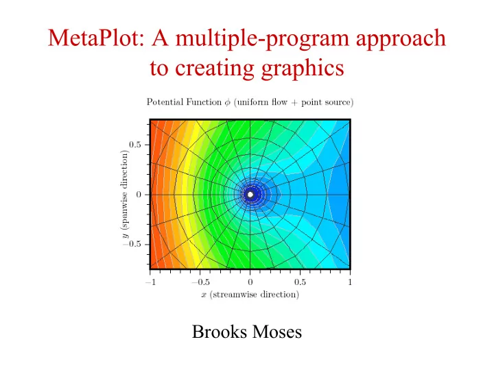
MetaPlot: A multiple-program approach to creating graphics Brooks Moses What do we want in a data plot? The data should be shown in the manner we desire. The presentation should be print-quality. Why not use an off-the-shelf solution?


slide-1
SLIDE 1

MetaPlot: A multiple-program approach to creating graphics

Brooks Moses

slide-2
SLIDE 2

What do we want in a data plot?

  • The data should be shown in the manner we desire.
  • The presentation should be print-quality.
slide-3
SLIDE 3

Why not use an off-the-shelf solution?

  • We may not be able to find a program that produces

exactly the type of plot we want.

  • Many programs cannot produce plots that use the

same fonts as our TeX documents.

  • In many programs, it is difficult to produce a plot of

a desired on-page size without rescaling the fonts and line widths.

  • Most high-quality plot programs are commercial, and

tend to be relatively expensive.

  • Conclusion: If we want it done right, we may have to

write (at least part of) it ourselves.

slide-4
SLIDE 4

Pros and Cons of Language Choices.

  • MetaPost:
  • uses TeX directly for label formatting.
  • has a simple and very powerful interface for creating

graphic elements, and the output process is built-in.

  • but is not well-suited to complicated math.
  • Programs in “traditional” languages (such as C++):
  • can deal with complicated math or algorithms easily.
  • may be able to use existing code libraries.
  • but do not come with a built-in interface for creating

graphic elements or labels, and require the user to consider the details of creating Postscript output.

slide-5
SLIDE 5

Proposal: Combine the strengths of both.

  • Instead of doing all of the work of creating a plot in
  • ne language, we can divide the process up into

parts, and do each part in the language that works best for it.

  • Thus, the key idea of MetaPlot:
  • Generate the “core plot” in a C++ program (or a

Fortran program, or something similar).

  • Scale the plot to the desired size, adjust the line

widths, and add annotations in MetaPost.

slide-6
SLIDE 6

What constitutes the “core plot”?

  • The C++ program is responsible for creating the

“core plot”: an abstract representation of the plot that is independent of its realization on the page.

  • In the contour-plot example,

the core plot consists of the shapes and colors of the contours and the shape of the grid, but not the line widths or the annotations.

slide-7
SLIDE 7

Conceptual design of the core plot.

  • Data transfer is via a partial MetaPost file containing

variable definitions.

  • The plot components are stored in separate picture

variables.

slide-8
SLIDE 8

Scaling of core-plot elements

  • Each plot element is defined to fit within the unit

square.

  • Actual data dimensions are stored separately, where

they are less subject to MetaPost’s number size limitations.

contplotA.xleft = -1.0; contplotA.xright = 1.0; contplotA.ybot = -0.75; contplotA.ytop = 0.75;

slide-9
SLIDE 9

Structure of a core-plot file.

  • As a more extended example, this is what a core-plot

file looks like:

contplotA.xleft = -1.0; contplotA.xright = 1.0; contplotA.ybot = -0.75; contplotA.ytop = 0.75; picture contplotA.grid; contplotA.grid := nullpicture; addto contplotA.grid doublepath (0.48,0.5)--(0.47,0.5); addto contplotA.grid doublepath (0.47,0.5)--(0.46,0.5); [...] picture contplotA.fillplot; contplotA.fillplot := nullpicture; addto contplotA.fillplot contour (0.48,0.5)--(0.47,0.5)

  • -(0.47,0.51)--(0.48,0.51)--cycle;

[...]

slide-10
SLIDE 10

Types of data structures in MetaPlot

  • Core-plot data structure
  • The core-plot data structure contains the abstracted

plot information, as just described.

  • Plot-instance data structure.
  • The plot-instance data structure is created in MetaPlot

from a core-plot data structure, and contains the information required to create a plot on the page:

  • Locations of the corners of the plot in the figure

coordinates.

  • Copies of the plot’s data scale information.
  • A macro that references the plot details from a core-

plot data structure.

slide-11
SLIDE 11

Some comments on plot scaling

  • The plot-instance’s page locations are stored as
  • rdinary MetaPost variables, and can be used in

linear equations.

  • For example, consider the definitions of pagewidth

and pageheight, and the plot_setequalaxes macro:

inst.pagewidth = inst.pageright - inst.pageleft; inst.pageheight = inst.pagetop - inst.pagebottom; def plot_setequalaxes(suffix inst) = inst.pagewidth = inst.pageheight * (inst.scalewidth/inst.scaleheight); enddef;

slide-12
SLIDE 12

Example: Creation of the title image, step 0.

  • Before we start, we need to have a plot-object file.

This one was created with a very early version of MetaContour, which is a general-purpose contour- plot program that I’m writing.

  • The input files will look something like this:

TITLE="Potential-Flow Contour Plot" VARIABLES="x" "y" "phi" ZONE I=32 J=16 0.11750 0.50000 0.61235 0.21500 0.50000 0.44262 0.29750 0.50000 0.25754 0.36500 0.50000 0.35465 0.41750 0.50000 0.44829 [...]

slide-13
SLIDE 13

Example: Creation of the title image, step 1.

  • To start with, a fairly basic preamble defining some

line sizes and creating the plot instance.

prologues:=0; input metaplot % metaplot macros input mc-color % plot-object file pen thickline; thickline := pencircle scaled 2pt; pen thinline; thinline := pencircle scaled 1pt; pen hairline; hairline := pencircle scaled 0.25pt; plot_instantiate(cplotA, contplotA); cplotA.pagewidth = 4.0in; plot_setequalaxes(cplotA); cplotA.llft = (0,0);

slide-14
SLIDE 14

Example: Creation of the title image, step 2.

  • Start with the basic filled plot:

draw cplotA.plot(FillPlot);

slide-15
SLIDE 15

Example: Creation of the title image, step 3.

  • Next, add the lineplot lines in light gray to delineate

the edges of the contours more clearly.

draw cplotA.plot(LinePlot) withpen hairline withcolor 0.75white;

slide-16
SLIDE 16

Example: Creation of the title image, step 4.

  • Add the grid lines, in a dark gray.

draw cplotA.plot(Grid) withpen hairline withcolor 0.25white;

slide-17
SLIDE 17

Example: Creation of the title image, step 5.

  • Draw a border around the plot area.

linejoin:=mitered; draw cplotA.llft--cplotA.lrt--cplotA.urt--cplotA.ulft--cycle withpen thickline;

slide-18
SLIDE 18

Example: Creation of the title image, step 6.

  • Put the numbered major grid ticks on the x-axis.

draw plot_xtickscale(cplotA)(cplotA.llft, cplotA.lrt, 0.08in, 0.06in, down, 0.0, 0.5, "%3f") withpen thinline;

slide-19
SLIDE 19

Example: Creation of the title image, step 7.

  • Put the unnumbered minor grid ticks on the x-axis.

draw plot_xtickscale(cplotA)(cplotA.llft, cplotA.lrt, 0.05in, 0.06in, down, 0.0, 0.1, "") withpen thinline;

slide-20
SLIDE 20

Example: Creation of the title image, step 8.

  • Put similar grid ticks on the y-axis.

draw plot_ytickscale(cplotA)(cplotA.llft, cplotA.ulft, 0.05in, 0.06in, left, 0.0, 0.1, "") withpen thinline;

slide-21
SLIDE 21

Example: Creation of the title image, step 9.

  • Define picture variables containing the axis labels

and title, using TeX for the text formatting.

picture xname; xname := btex $x$ (streamwise direction) etex; picture yname; yname := btex $y$ (spanwise direction) etex rotated 90; picture plottitle; plottitle := btex Potential Function $\phi$ (uniform flow $+$ point source) etex;

slide-22
SLIDE 22

Example: Creation of the title image, step 10.

  • Place the various labels on the plot, using the macros

for placing axis tickmarks.

draw axes_ticklabeled(0.5[cplotA.llft,cplotA.lrt], 0.0, 0.3125in, down, xname); draw axes_ticklabeled(0.5[cplotA.llft,cplotA.ulft], 0.0, 0.3125in, left, yname);

slide-23
SLIDE 23

Example: Creation of the title image, step 11.

  • Finally, place the title at the top of the plot.

draw axes_ticklabeled(0.5[cplotA.ulft,cplotA.urt], 0.0, 0.1875in, up, plottitle);