Measures of Spread The population Variance , 2 , measures each - - PowerPoint PPT Presentation

Unit 1: Introduction to data Lecture 3: EDA (cont.) and Introduction to statistical inference via simulation Statistics 101

Nicole Dalzell May 15, 2015

Spread

Measures of Spread

The population Variance, σ2, measures each observation’s deviation from the mean. The population Standard Deviation, σ, is the square root of the variance. The Inner Quartile Range (IQR) measures the spread of the middle 50% of your data, and is visually depicted in Boxplots.

Link Statistics 101 ( Nicole Dalzell) U1 - L3: EDA + Inference May 15, 2015 2 / 1 Spread

Box Plot

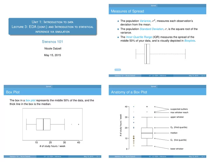
The box in a box plot represents the middle 50% of the data, and the thick line in the box is the median.

# of study hours / week 10 20 30 40

Statistics 101 ( Nicole Dalzell) U1 - L3: EDA + Inference May 15, 2015 3 / 1 Spread

Anatomy of a Box Plot

# of study hours / week 10 20 30 40 lower whisker Q1 (first quartile) median Q3 (third quartile) upper whisker max whisker reach suspected outliers

Statistics 101 ( Nicole Dalzell) U1 - L3: EDA + Inference May 15, 2015 4 / 1

Spread

Measures of Location

The 25th percentile is also called the first quartile, Q1. The 50th percentile is also called the median. The 75th percentile is also called the third quartile, Q3.

summary( d$study hours ) Min . 1 st Qu. Median Mean 3rd Qu. Max. NAs 3.00 10.00 15.00 17.42 20.00 40.00 13.00 Between Q1 and Q3 is the middle 50% of the data. The range these data span is called the interquartile range, or the IQR. IQR = 20 − 10 = 10

Statistics 101 ( Nicole Dalzell) U1 - L3: EDA + Inference May 15, 2015 5 / 1 Spread

Whiskers and Outliers

Whiskers of a box plot can extend up to 1.5 * IQR away from the quartiles.

max upper whisker reach : Q3 + 1.5 ∗ IQR = 20 + 1.5 ∗ 10 = 35 max lower whisker reach : Q1 − 1.5 ∗ IQR = 10 − 1.5 ∗ 10 = −5

An outlier is defined as an observation beyond the maximum reach of the whiskers. It is an observation that appears extreme relative to the rest of the data.

Statistics 101 ( Nicole Dalzell) U1 - L3: EDA + Inference May 15, 2015 6 / 1 Spread

Outliers (cont.)

Why is it important to look for outliers? Identify extreme skew in the distribution. Identify data collection and entry errors. Provide insight into interesting features of the data.

Statistics 101 ( Nicole Dalzell) U1 - L3: EDA + Inference May 15, 2015 7 / 1 Spread

Why visualize?

What does a response of 0 mean in this distribution?

• 2

4 6 8 10 12

Number of drinks it takes students to get drunk

Statistics 101 ( Nicole Dalzell) U1 - L3: EDA + Inference May 15, 2015 8 / 1

Spread Robust Statistics

Extreme observations

How would sample statistics such as mean, median, SD, and IQR of household income be affected if the largest value was replaced with $10 million? What if the smallest value was replaced with $10 million?

household income ($ thousands) 200 400 600 800 1000

• ●
• Statistics 101 ( Nicole Dalzell)

U1 - L3: EDA + Inference May 15, 2015 9 / 1 Spread Robust Statistics

Income Example

household income ($ thousands) 200 400 600 800 1000

• ●
• robust

not robust scenario median IQR

¯

x s

• riginal data

165K 150K 211K 180K move largest to $10 million 165K 150K 398K 1,422K move smallest to $10 million 190K 163K 4,186K 1,424K

Statistics 101 ( Nicole Dalzell) U1 - L3: EDA + Inference May 15, 2015 10 / 1 Spread Robust Statistics

Robust statistics

Since the median and IQR are more robust to skewness and outliers than mean and SD: skewed → median and IQR symmetric → mean and SD If you were searching for a car, and you are price conscious, would you be more interested in the mean or median vehicle price when con- sidering a car?

Statistics 101 ( Nicole Dalzell) U1 - L3: EDA + Inference May 15, 2015 11 / 1 Spread Robust Statistics

Range and IQR

Range Range of the entire data. range = max − min IQR Range of the middle 50% of the data. IQR = Q3 − Q1 Is the range or the IQR more robust to outliers?

Statistics 101 ( Nicole Dalzell) U1 - L3: EDA + Inference May 15, 2015 12 / 1

Spread Robust Statistics

Example: Visualizing

What does our Energy Data look like?

5000 10000 15000

Energy Use Data Boxplot

Energy Usage

Statistics 101 ( Nicole Dalzell) U1 - L3: EDA + Inference May 15, 2015 13 / 1 Spread Robust Statistics

Who uses the most energy?

Country.Name X2011 1 Iceland 17964.44 2 Qatar 17418.69 3 Trinidad and Tobago 15691.29 4 Kuwait 10408.28 5 Brunei Darussalam 9427.09 6 Oman 8356.29 7 Luxembourg 8045.90 8 United Arab Emirates 7407.01 9 Bahrain 7353.16 10 Canada 7333.28 11 North America 7062.22 12 United States 7032.35 13 Saudi Arabia 6738.42 14 Singapore 6452.33 15 Finland 6449.04

Statistics 101 ( Nicole Dalzell) U1 - L3: EDA + Inference May 15, 2015 14 / 1 Spread Robust Statistics

Participation question Which of the following is false about the distribution of average number

• f hours students study daily?
• 2

4 6 8 10

Average number of hours students study daily

• Min. 1st Qu.

Median Mean 3rd Qu. Max. 1.000 3.000 4.000 3.821 5.000 10.000 (a) There are no students who don’t study at all. (b) 75% of the students study more than 5 hours daily, on average. (c) 25% of the students study less than 3 hours, on average. (d) IQR is 2 hours.

Statistics 101 ( Nicole Dalzell) U1 - L3: EDA + Inference May 15, 2015 15 / 1 Spread Robust Statistics

Side-by-side box plot

How does the number of the average number of times students go

• ut per week vary by involvement? Do the two variables appear to be

associated or independent?

• Greek

Independent SLG 1 2 3 4 5 Statistics 101 ( Nicole Dalzell) U1 - L3: EDA + Inference May 15, 2015 16 / 1

Spread Robust Statistics

Measures of Spread

The population Variance, σ2, measures each observation’s deviation from the mean. The population Standard Deviation, σ, is the square root of the variance. The Inner Quartile Range (IQR) measures the spread of the middle 50% of your data, and is visually depicted in Boxplots.

Link Statistics 101 ( Nicole Dalzell) U1 - L3: EDA + Inference May 15, 2015 17 / 1 Spread Deviation

Deviation

The distance of an observation from the mean is its deviation: xi − ¯ x.

sort ( d$sleep ) [ 1 ] 1 1 2 2 2 3 3 3 3 3 3 3 3 3 3 3 3 3 3 3 3 3 3 3 3 3 3 3 3 [30] 4 4 5 5 5 5 5 5 5 5 5 5 5 5 5 5 5 5 5 5 5 5 5 5 5 5 5 5 5 [59] 5 5 5 5 5 5 5 5 5 5 5 5 5 5 6 6 7 7 7 7 7 7 7 7 8 9 9 9 mean( d$sleep ) [ 1 ] 4.6

x1 − ¯ x = 1 − 4.6 = −3.6 x2 − ¯ x = 1 − 4.6 = −3.6 x3 − ¯ x = 2 − 4.6 = −2.6

. . .

x86 − ¯ x = 9 − 4.6 = 4.4

Statistics 101 ( Nicole Dalzell) U1 - L3: EDA + Inference May 15, 2015 18 / 1 Spread Deviation

Variance

Population Variance, σ2 Roughly the average squared deviation from the mean

σ2 = N

i=1(xi − µ)2

N

Statistics 101 ( Nicole Dalzell) U1 - L3: EDA + Inference May 15, 2015 19 / 1 Spread Deviation

Variance (cont.)

Why do we use the squared deviation in the calculation of variance? To get rid of negatives so that observations equally distant from the mean are weighed equally. To weigh larger deviations more heavily

Statistics 101 ( Nicole Dalzell) U1 - L3: EDA + Inference May 15, 2015 20 / 1

Spread Deviation

Variance

Sample Variance, s2 Roughly the average squared deviation from the mean s2 =

n

i=1(xi − ¯

x)2 n − 1 Given that the sample mean is 4.6, the sample variance of the hours

• f sleep students get per night can be calculated as:

s2 = (1 − 4.6)2 + (1 − 4.6)2 + · · · + (9 − 4.6)2 86 − 1

= 2.76

Statistics 101 ( Nicole Dalzell) U1 - L3: EDA + Inference May 15, 2015 21 / 1 Spread Deviation

Notation Recap

mean variance SD sample

¯

x s2 s population

µ σ2 σ

Do you see a trend in what types of letters are used for sample statistics vs. population parameters? Latin letters for sample statistics, Greek letters for population parameters.

Statistics 101 ( Nicole Dalzell) U1 - L3: EDA + Inference May 15, 2015 22 / 1 Spread Deviation

Application exercise: Variability

Statistics 101 ( Nicole Dalzell) U1 - L3: EDA + Inference May 15, 2015 23 / 1 Spread Deviation

Variability vs. diversity

Which of the following sets of cars has more diverse composition of colors? Set 1: Set 2:

Statistics 101 ( Nicole Dalzell) U1 - L3: EDA + Inference May 15, 2015 24 / 1

Spread Deviation

Variability vs. diversity (cont.)

Which of the following sets of cars has more variable mileage? Set 1:

10 20 30 40 50 60

less variable

1 2 3

Set 2:

10 20 30 40 50 60

more variable

1 2 3

Statistics 101 ( Nicole Dalzell) U1 - L3: EDA + Inference May 15, 2015 25 / 1 Spread Standard Deviation

Standard deviation

Standard deviation, s Roughly the deviation around the mean, calculated as the square root

• f the variance, and has the same units as the data.

s =

• s2 =

n

i=1(xi − ¯

x)2 n − 1

The standard deviation of the number of hours the students slept is: s = √ 2.759 ≈ 1.66

Statistics 101 ( Nicole Dalzell) U1 - L3: EDA + Inference May 15, 2015 26 / 1 Spread Standard Deviation

Standard Deviation

The standard deviation gives a rough estimate of the typical distance of a data point from the mean. The larger the standard deviation, the more variability there is in the data and the more spread out the data are.

Standard Deviation of 2

rnorm(1000,0,2) Frequency −15 −10 −5 5 10 15 50 100 150 200

Standard Deviation of 4

rnorm(1000,0,4) Frequency −15 −10 −5 5 10 15 50 100 150 200

Statistics 101 ( Nicole Dalzell) U1 - L3: EDA + Inference May 15, 2015 27 / 1 Variability and Z-scores

Variability in Student Sleep

sleep, x = 4.6, sx = 1.66 2 4 6 8

• 69 out of 86 students (80%) are within 1 SD of the mean.

80 out of 86 students (93%) are within 2 SDs of the mean. 86 out of 86 students (100%) are within 3 SDs of the mean.

Statistics 101 ( Nicole Dalzell) U1 - L3: EDA + Inference May 15, 2015 28 / 1

Variability and Z-scores

95% Rule

95 % Rule If a distribution of data is approximately symmetric and bell-shaped, about 95% of the data should fall within two standard deviations of the mean. For a population, 95% of the data will be between µ − 2σ and

µ + 2σ

http://rchsbowman.files.wordpress.com/2008/09/empirical-rule-3.jpg

Statistics 101 ( Nicole Dalzell) U1 - L3: EDA + Inference May 15, 2015 29 / 1 Variability and Z-scores

Z-Scores

Z-Score The z-score for a data value, xi , is z = xi − ¯ x s For a population, ¯ x is replaced with µ and s is replaced with σ. Values farther from 0 are more extreme.

Statistics 101 ( Nicole Dalzell) U1 - L3: EDA + Inference May 15, 2015 30 / 1 Variability and Z-scores

Z-Scores: Why?

A z-score puts values on a common scale A z-score is the number of standard deviations a value falls from the mean 95% of all z-scores fall between -2 and 2 . z-scores beyond -2 or 2 can be considered extreme

Statistics 101 ( Nicole Dalzell) U1 - L3: EDA + Inference May 15, 2015 31 / 1 Variability and Z-scores

Z-Scores: Example

Which is better, (A) an ACT score of 28 or (B) a combined SAT score

• f 2100 ?

ACT: ¯ x = 21, s = 5 SAT: ¯ x = 1500, s = 325

ACT: z = 28 − 21 5

= 7

5 = 1.4 SAT: z = 2100 − 1500 325

= 600

325 = 1.85

Histogram of Z−Scores

Z−Score Frequency −3 −2 −1 1 2 3 100 200 300

Statistics 101 ( Nicole Dalzell) U1 - L3: EDA + Inference May 15, 2015 32 / 1

Categorical Variables Relationship between two categorical variables

Mosaic plots

A survey question asked students, “Have you ever used Adderall for an exam or to study?” Based on their responses, does there appear to be a relationship between gender and having used Adderall for an exam or to study?

female male no yes

% female who used Adderall < % males

Statistics 101 ( Nicole Dalzell) U1 - L3: EDA + Inference May 15, 2015 33 / 1 Categorical Variables Relationship between two categorical variables

Contingency table and mosaic plot

In 1973, the University of California-Berkeley was sued for sex

• discrimination. The numbers looked pretty incriminating: the graduate

schools had just accepted 44% of male applicants but only 35% of female applicants. Admit Deny Total Male 3738 4704 8442 Female 1494 2827 4321 Total 5232 7531 12763 % Males admitted: 3738 / 8442 = 44% % Females admitted: 1494 / 4321 = 35%

status

female male admit deny

Statistics 101 ( Nicole Dalzell) U1 - L3: EDA + Inference May 15, 2015 34 / 1 Categorical Variables Relationship between two categorical variables

Further analysis of these data:

“If the data are properly pooled...there is a small but statistically significant bias in favor of women.”

Bickel, P . J., Hammel, E. A., & O’Connell, J. W. (1975). Sex bias in graduate admissions: Data from Berkeley. Science, 187(4175), 398-404. http://www.unc.edu/ ∼nielsen/soci708/cdocs/Berkeley admissions bias.pdf Statistics 101 ( Nicole Dalzell) U1 - L3: EDA + Inference May 15, 2015 35 / 1 Categorical Variables Relationship between two categorical variables

Proper pooling

Let’s take a closer look at the top 6 departments: vs. Play with it at http://vudlab.com/simpsons .

Statistics 101 ( Nicole Dalzell) U1 - L3: EDA + Inference May 15, 2015 36 / 1

Categorical Variables Relationship between two categorical variables

Simpson’s paradox

Every Simpson’s paradox involves at least three variables:

1

the response variable (accepted/not accepted)

2

the observed explanatory variable (male/ female)

3

the lurking explanatory variable (what department did you apply to) If the effect of the observed explanatory variable on the response variable changes directions when you account for the lurking explanatory variable, you’ve got a Simpson’s Paradox.

Statistics 101 ( Nicole Dalzell) U1 - L3: EDA + Inference May 15, 2015 37 / 1