= + + Max R 2 x 4 x Max R rx ... r x 1 2 x 1 1 n n - - PDF document

1

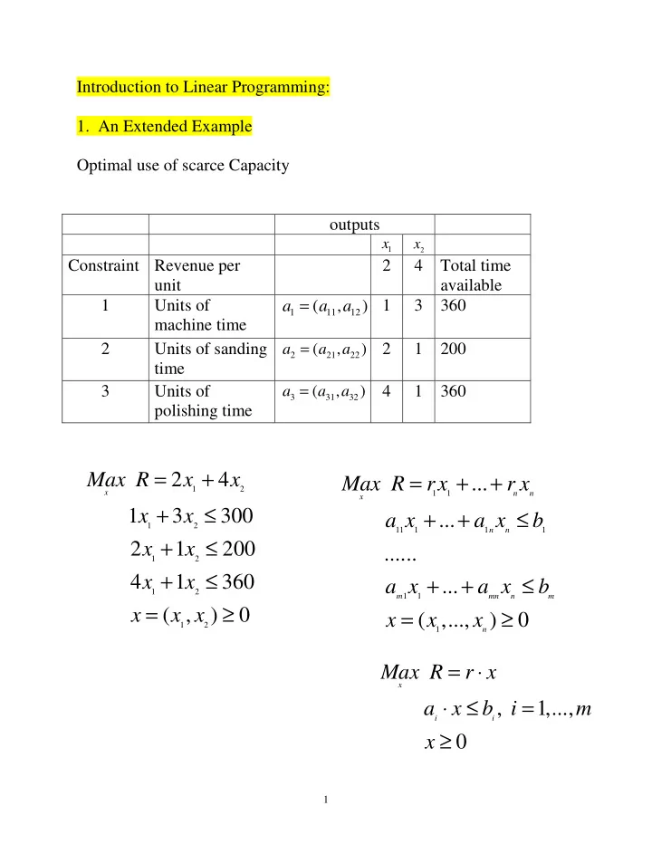
Introduction to Linear Programming:

• 1. An Extended Example

Optimal use of scarce Capacity

• utputs

1

x

2

x

Constraint Revenue per unit 2 4 Total time available 1 Units of machine time

1 11 12

( , ) a a a = 1 3 360 2 Units of sanding time

2 21 22

( , ) a a a =

2 1 200 3 Units of polishing time

3 31 32

( , ) a a a =

4 1 360

, 1,...,

x i i

Max R r x a x b i m x = ⋅ ⋅ ≤ = ≥

1 2 1 2 1 2 1 2 1 2

2 4 1 3 300 2 1 200 4 1 360 ( , )

x

Max R x x x x x x x x x x x = + + ≤ + ≤ + ≤ = ≥

1 1 11 1 1 1 1 1 1

... ... ...... ... ( ,..., )

n n x n n m mn n m n

Max R rx r x a x a x b a x a x b x x x = + + + + ≤ + + ≤ = ≥

2

Constant revenue line

1 2

2 4 x x R + =

has slope

1 2 m = −

1 2 1 2 1 2 1 2 1 2

2 4 1 3 300 2 1 200 4 1 360 ( , )

x

Max R x x x x x x x x x x x = + + ≤ + ≤ + ≤ = ≥

100

i

m = slope of constraint i.

90

1

x

2

x

(60,80) (80,40)

3

4 m = −

2

2 m = −

1 1 3

m = −

3

Consider the effect of relaxing the second constraint

1 2 1 2 2

3 300 2 x x x x b + = + =

1 2 1 2 2 1 2

3 300 6 3 3 __________ 5 3 300 x x x b x b + = + = = −

3 1 2 5

60 x b = −

,

1 2 2 1 2 5

2 120 x b x b = − = −

3 1 1 2 5 5

2 4 2( 60) 4(120 ) R x x b b = + = − + −

2 2 5 2

R b λ ∂ = = ∂

100 90

1

x

2

x

(60,80) (80,40)

3

4 m = − 2

i

shadow value of resource λ =

3

λ =

4

Imputed prices/ shadow prices (Lagrange Multipliers)

* 1

imputed price forconstraint

i n ij j j j

i a x b λ

=

= ≤ ∑

Value of relaxing the constraint so

* i

λ ≥

* i

λ = value to firm of an additional unit of capacity

= extra revenue that the firm would get = cost to firm if it had to give up a unit of capacity Shadow prices are "as if" prices which support the optimum. What does this mean? Think of the profit maximizing decision as if these were actual prices.

* 1 1 1 1 2 3

If 0 then 0, that is 2 1 2 4 x MR MC λ λ λ > − = − − − =

.

* 1 1 1 1 2 3

If 0 then 0, that is 2 1 2 4 x MR MC λ λ λ = − ≤ − − − ≤

.

* 2 2 2 1 2 3

If 0 then 0, that is 4 3 1 1 x MR MC λ λ λ > − = − − − =

.

* 2 2 2 1 2 3

If 0 then 0, that is 4 3 1 1 x MR MC λ λ λ = − ≤ − − − ≤

.

5

We already know that the third constraint is not binding so

* 3

λ = . We also know that the optimal levels of outputs 1 and 2 are positive. Thus for these outputs MR = MC and so

* * 1 2

2 1 2 λ λ − − =

and

* * 1 2

4 3 1 λ λ − − =

.

1 2 1 2

2 2 3 4 λ λ λ λ + = + = ,

1 2 1 2 1

2 2 6 2 8 _________ 5 6 λ λ λ λ λ + = + = =

Hence

* 6 1 5

λ = and

* 2 2 5

λ =

6

We now look at the general programming problem . Programming problem

1 n j j j

Maximize r x

=

∑

subject to the constraints

1 n ij j i j

a x b

=

≤

∑

and

1

( ,..., )

n

x x x = ≥ Valuing total output aij = amount of input i needed to produce a unit of output j. ( ,..., ) 1 x x xn = an n-vector of outputs. ( ,..., ) 1 m λ λ λ = an m-vector of non-negative (shadow) prices, one for each input. We seek shadow prices

1

( ,..., )

m

λ λ λ = which will “support” the optimal

• utput plan.

7

Necessary condition: No Marginal profit (otherwise firm could make an infinite profit by increasing output) For output j

j j

MR r =

1 m j i ij i

MC a λ

=

=∑ . We require

j j

MC MR ≥ Thus we consider only non-negative shadow prices for which

1 m i ij j i

a r λ

=

≥

∑

If

j j

MC MR = the total profit from producing product j is

* 1

( )

m j i ij j i

r a x λ

=

− =

∑

The other possibility is

j j

MC MR > in which case

* j

x = thus again the total profit from producing product j is zero. Since this holds for all products we have the following Proposition. Proposition: If shadow prices support the maximum the total revenue equals total “shadow” cost.

8

Fundamental Theorem of Linear Programming There exists a vector of shadow prices

* * * 1

( ,..., )

m

λ λ λ = which supports the optimal output vector

*

x .