matched and nested case control studies
play

Matched and nested case-control studies Bendix Carstensen Steno - PDF document

Matched and nested case-control studies Bendix Carstensen Steno Diabetes Center, Gentofte, Denmark b@bxc.dk http://BendixCarstensen.com Department of Biostatistics, University of Copenhagen, 18 November 2016


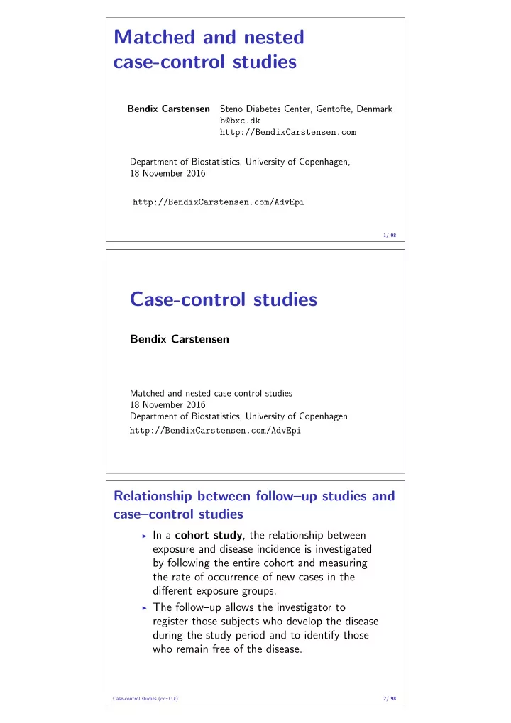
  1. Matched and nested case-control studies Bendix Carstensen Steno Diabetes Center, Gentofte, Denmark b@bxc.dk http://BendixCarstensen.com Department of Biostatistics, University of Copenhagen, 18 November 2016 http://BendixCarstensen.com/AdvEpi 1/ 98 Case-control studies Bendix Carstensen Matched and nested case-control studies 18 November 2016 Department of Biostatistics, University of Copenhagen http://BendixCarstensen.com/AdvEpi Relationship between follow–up studies and case–control studies ◮ In a cohort study , the relationship between exposure and disease incidence is investigated by following the entire cohort and measuring the rate of occurrence of new cases in the different exposure groups. ◮ The follow–up allows the investigator to register those subjects who develop the disease during the study period and to identify those who remain free of the disease. Case-control studies ( cc-lik ) 2/ 98

  2. Relationship between follow–up studies and case–control studies ◮ In a case-control study the subjects who develop the disease (the cases) are registered by some other mechanism than follow-up ◮ A group of healthy subjects (the controls) is used to represent the subjects who do not develop the disease. ◮ Persons are selected on the basis of disease outcome . ◮ Occasionally referred to as “retrospective study” . Case-control studies ( cc-lik ) 3/ 98 Rationale behind case-control studies ◮ In a follow-up study, rates among exposed and non-exposed are estimated by: D 1 D 0 and Y 1 Y 0 ◮ and the rate ratio by: � D 0 � Y 1 D 1 = D 1 Y 1 Y 0 D 0 Y 0 Case-control studies ( cc-lik ) 4/ 98 Rationale behind case-control studies ◮ Case-control study: same cases but controls represent the distribution of risk time H 1 ≈ Y 1 H 0 Y 0 ◮ . . . therefore the rate ratio is estimated by: � H 1 D 1 D 0 H 0 ◮ Controls represent risk time , not disease-free persons. Case-control studies ( cc-lik ) 5/ 98

  3. Case–control probability tree Exposure Failure Selection Probability ✟✟✟✟ s 1 = 0 . 97 Case p π 1 × 0 . 97 ( D 1 ) ✑✑✑✑ π 1 ❍❍❍❍ F 0 . 03 E 1 ◗◗◗◗ ✟✟✟✟ k 1 = 0 . 01 Control p p (1 − π 1 ) × 0 . 01 � ( H 1 ) � ❍❍❍❍ 1 − π 1 S � � 0 . 99 ✟✟✟✟ ❅ Case s 0 = 0 . 97 (1 − p ) π 0 × 0 . 97 ❅ ( D 0 ) π 0 ✑✑✑✑ ❍❍❍❍ ❅ F ❅ 1 − p 0 . 03 E 0 ◗◗◗◗ ✟✟✟✟ Control k 0 = 0 . 01 (1 − p )(1 − π 0 ) × 0 . 01 ( H 0 ) ❍❍❍❍ 1 − π 0 S 0 . 99 Case-control studies ( cc-lik ) 6/ 98 What is estimated by the case-control ratio? = 0 . 97 π 1 � s 1 π 1 � D 1 0 . 01 × = × 1 − π 1 1 − π 1 H 1 k 1 = 0 . 97 π 0 � s 0 π 0 � D 0 0 . 01 × = × 1 − π 0 1 − π 0 H 0 k 0 D 1 / H 1 = π 1 / (1 − π 1 ) π 0 / (1 − π 0 ) = OR population D 0 / H 0 — but only for equal sampling fractions: s 1 / k 1 = s 0 / k 0 ⇐ s 1 = s 0 ∧ k 1 = k 0 . Case-control studies ( cc-lik ) 7/ 98 Estimation from case-control study Odds-ratio of disease between exposed and unexposed given inclusion : � OR = ω 1 π 1 π 0 = ω 0 1 − π 1 1 − π 0 odds-ratio of disease (for a small interval) between exposed and unexposed in the study is the same as odds-ratio for disease between exposed and unexposed in the “study base” , Case-control studies ( cc-lik ) 8/ 98

  4. Estimation from case-control study . . . under the assumption that: ◮ inclusion probability is the same for exposed and unexposed cases. ◮ inclusion probability is the same for exposed and unexposed controls. The selection mechanism can only depend on case/control status. Case-control studies ( cc-lik ) 9/ 98 Disease OR and exposure OR ◮ The disease -OR comparing exposed and non-exposed given inclusion in the study is the same as the population-OR: � D 0 π 1 � π 0 D 1 = = OR pop H 1 H o 1 − π 1 1 − π 0 ◮ The disease -OR is equal to the exposure -OR comparing cases and controls: � D 0 � H 1 D 1 = D 1 = D 1 H 0 H 1 H o D o H o D 0 H 1 Case-control studies ( cc-lik ) 10/ 98 Log-likelihood for case-control studies The observations in a case-control study are ◮ Response: case/control status ◮ Covariates: exposure status, etc. Parameters possible to estimate are odds of disease conditional on inclusion into the study. and therefore also odds ratio of disease between groups conditional on inclusion into the study. Case-control studies ( cc-lik ) 11/ 98

  5. Log-likelihood for case-control studies The log-likelihood is a binomial likelihood with odds of being a case (conditional on being included): ◮ odds ω 0 for unexposed and ◮ odds ω 1 for exposed or ◮ odds ω 0 for unexposed and ◮ the odds-ratio θ = ω 1 /ω 0 between exposed and unexposed. Only the odds-ratio parameter, θ , is of interest Case-control studies ( cc-lik ) 12/ 98 Log-likelihood for case-control studies Case/control outcome and exposure ( 0 / 1 ): ◮ unexposed group: N 0 persons, D 0 cases, N 0 − D 0 controls, case-odds ω 0 ◮ exposed group: N 1 persons, D 1 cases, N 1 − D 1 controls, case-odds ω 1 = θω 0 Binomial log-likelihood: D 0 ln( ω 0 ) − N 0 ln(1+ ω 0 )+ D 1 ln( θω 0 ) − N 1 ln(1+ θω 0 ) — logistic regression with case/control status as outcome and exposure as explanatory variabale Case-control studies ( cc-lik ) 13/ 98 Log-likelihood for case-control studies Binomial outcome (case/control) and binary exposure ( 0 / 1 ) Odds-ratio ( θ ) is the ratio of ω 1 to ω 0 , so: ln( θ ) = ln( ω 1 /ω 0 ) = ln( ω 1 ) − ln( ω 0 ) Estimates of ln( ω 1 ) and ln( ω 0 ) are: � D 1 � � D 0 � � � ln( ω 1 ) = ln and ln( ω 0 ) = ln H 1 H 0 Case-control studies ( cc-lik ) 14/ 98

  6. Log-likelihood for case-control studies Estimated log-odds have standard errors: � � 1 + 1 1 + 1 and D 1 H 1 D 0 H 0 Exposed and unexposed form two independent bodies of data, so the estimate of ln( θ ) [= ln(OR)] is � � D 1 � � D 0 � 1 + 1 + 1 + 1 ln − ln , s.e. = H 1 H 0 D 1 H 1 D 0 H 0 Case-control studies ( cc-lik ) 15/ 98 BCG vaccination and leprosy New cases of leprosy were examined for presence or absence of the BCG scar. During the same period, a 100% survey of the population of this area, which included examination for BCG scar, had been carried out. BCG scar Leprosy cases Population survey Present 101 46,028 Absent 159 34,594 The tabulated data refer only to subjects under 35. What are the sampling fractions in this study? Case-control studies ( cc-lik ) 16/ 98 Odds ratio with confidence interval OR = D 1 / H 1 = 101 / 46 , 028 159 / 34 , 594 = 0 . 48 D 0 / H 0 � 1 + 1 + 1 + 1 s.e.(ln[OR]) = D 1 H 1 D 0 H 0 � 1 46 , 028 + 1 1 1 = 101 + 159 + 34 , 594 = 0 . 127 erf = exp(1 . 96 × 0 . 127) = 1 . 28 × × OR ÷ erf = 0 . 48 ÷ 1 . 28 = (0 . 37 , 0 . 61) ( 95% c.i. ) Case-control studies ( cc-lik ) 17/ 98

  7. Unmatched study with 1000 controls BCG scar Leprosy cases Controls Present 101 554 Absent 159 446 What are the sampling fractions here? OR = 101 / 554 159 / 446 = 0 . 1823 0 . 3565 = 0 . 51 � 101 + 1 1 554 + 1 159 + 1 s.e.(ln[OR]) = 446 = 0 . 142 erf = exp(1 . 96s.e.(ln[OR])) = 1 . 32 × 95% c.i.: 0 . 51 ÷ erf = (0 . 39 , 0 . 68) Case-control studies ( cc-lik ) 18/ 98 Frequency matched studies Bendix Carstensen Matched and nested case-control studies 18 November 2016 Department of Biostatistics, University of Copenhagen http://BendixCarstensen.com/AdvEpi Age-stratified odds-ratio: BCG data Exposure: BCG Potential confounder: age ◮ Age and BCG-scar correlated. ◮ Age is associated with leprosy. ◮ Bias in the estimation of the relationship between BCG-scar and leprosy. Estimate an OR for leprosy associated with BCG in each age-stratum. Combine to an overall estimate (if not too variable between strata). Frequency matched studies ( cc-str ) 19/ 98

  8. This is called stratified analysis (by age): Cases Population OR BCG − + − + estimate Age 0–4 1 1 7,593 11,719 0.65 5–9 11 14 7,143 10,184 0.89 10–14 28 22 5,611 7,561 0.58 15–19 16 28 2,208 8,117 0.48 20–24 20 19 2,438 5,588 0.41 25–29 36 11 4,356 1,625 0.82 30–34 47 6 5,245 1,234 0.54 Overall 0.58 Frequency matched studies ( cc-str ) 20/ 98 The simulated cc-study, stratified by age Cases Population BCG − + − + Age 0–4 1 1 101 137 5–9 11 14 91 115 10–14 28 22 82 101 15–19 16 28 28 87 20–24 20 19 25 69 25–29 36 11 63 21 30–34 47 6 56 24 Total 159 101 446 554 Frequency matched studies ( cc-str ) 21/ 98 Matching and efficiency ◮ If some strata have many controls per case and other only few, there is a tendency to“waste” ◮ controls in strata with many controls ◮ cases in strata with few controls ◮ The solution is to match or stratify the study design : ◮ Make sure that the ratio of cases to controls is approximately the same in all strata (e.g. age-groups). Frequency matched studies ( cc-str ) 22/ 98

Download Presentation
Download Policy: The content available on the website is offered to you 'AS IS' for your personal information and use only. It cannot be commercialized, licensed, or distributed on other websites without prior consent from the author. To download a presentation, simply click this link. If you encounter any difficulties during the download process, it's possible that the publisher has removed the file from their server.

Recommend


More recommend