Markov processes (Markov chains) Construct a Bayes net from these - - PDF document

SLIDE 1

Temporal probability models

Chapter 15, Sections 1–5

Chapter 15, Sections 1–5 1

Outline

♦ Time and uncertainty ♦ Inference: filtering, prediction, smoothing ♦ Hidden Markov models ♦ Dynamic Bayesian networks

Chapter 15, Sections 1–5 2

Time and uncertainty

The world changes; we need to track and predict it Diabetes management vs vehicle diagnosis Basic idea: copy state and evidence variables for each time step Xt = set of unobservable state variables at time t e.g., BloodSugart, StomachContentst, etc. Et = set of observable evidence variables at time t e.g., MeasuredBloodSugart, PulseRatet, FoodEatent This assumes discrete time; step size depends on problem Notation: Xa:b = Xa, Xa+1, . . . , Xb−1, Xb

Chapter 15, Sections 1–5 3

Markov processes (Markov chains)

Construct a Bayes net from these variables: parents? CPTs?

Chapter 15, Sections 1–5 4

Markov processes (Markov chains)

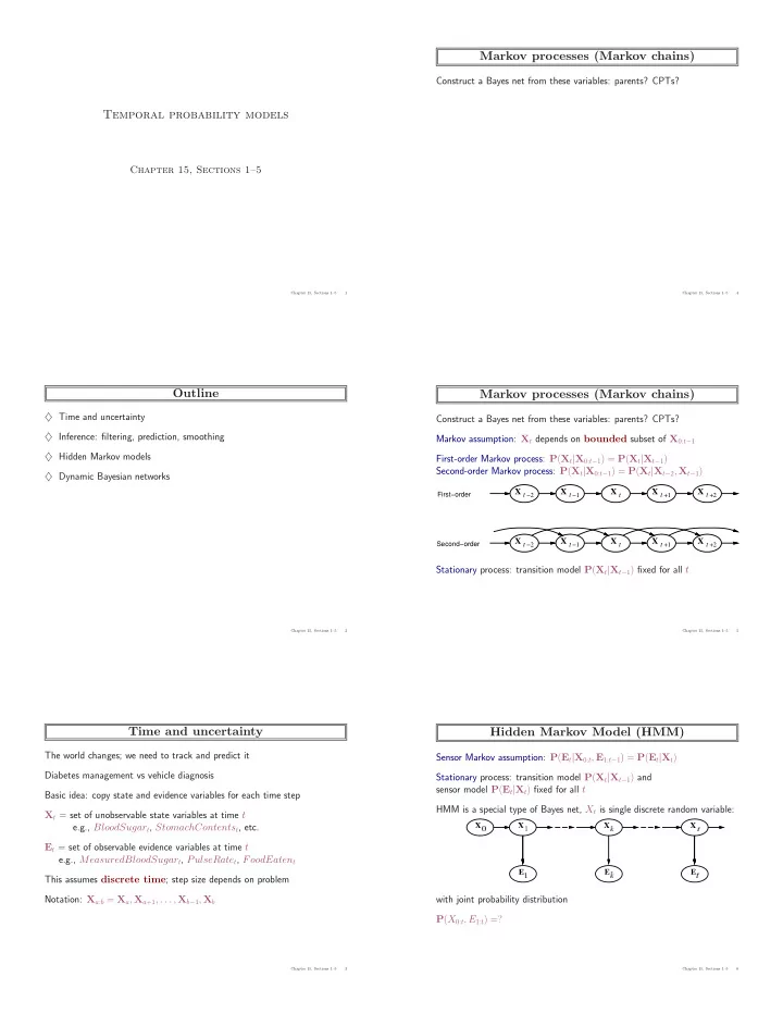
Construct a Bayes net from these variables: parents? CPTs? Markov assumption: Xt depends on bounded subset of X0:t−1 First-order Markov process: P(Xt|X0:t−1) = P(Xt|Xt−1) Second-order Markov process: P(Xt|X0:t−1) = P(Xt|Xt−2, Xt−1)

X t −1 X t X t −2 X t +1 X t +2 X t −1 X t X t −2 X t +1 X t +2

First−order Second−order

Stationary process: transition model P(Xt|Xt−1) fixed for all t

Chapter 15, Sections 1–5 5

Hidden Markov Model (HMM)

Sensor Markov assumption: P(Et|X0:t, E1:t−1) = P(Et|Xt) Stationary process: transition model P(Xt|Xt−1) and sensor model P(Et|Xt) fixed for all t HMM is a special type of Bayes net, Xt is single discrete random variable: with joint probability distribution P(X0:t, E1:t) =?

Chapter 15, Sections 1–5 6

SLIDE 2

Hidden Markov Model (HMM)

Sensor Markov assumption: P(Et|X0:t, E1:t−1) = P(Et|Xt) Stationary process: transition model P(Xt|Xt−1) and sensor model P(Et|Xt) fixed for all t HMM is a special type of Bayes net, Xt is single discrete random variable: with joint probability distribution P(X0:t, E1:t) = P(X0)Πt

i=1P(Xi|Xi−1)P(Ei|Xi)

Chapter 15, Sections 1–5 7

Example

t

Rain

t

Umbrella Raint −1 Umbrellat −1 Raint +1 Umbrellat +1

Rt −1

t

P(R ) 0.3 f 0.7 t

t

R

t

P(U ) 0.9 t 0.2 f

First-order Markov assumption not exactly true in real world! Possible fixes:

• 1. Increase order of Markov process
• 2. Augment state, e.g., add Tempt, Pressuret

Example: robot motion. Augment position and velocity with Batteryt

Chapter 15, Sections 1–5 8

Inference tasks

Filtering: P(Xt|e1:t) belief state—input to the decision process of a rational agent Prediction: P(Xt+k|e1:t) for k > 0 evaluation of possible action sequences; like filtering without the evidence Smoothing: P(Xk|e1:t) for 0 ≤ k < t better estimate of past states, essential for learning Most likely explanation: arg maxx1:t P(x1:t|e1:t) speech recognition, decoding with a noisy channel

Chapter 15, Sections 1–5 9

Filtering

Aim: devise a recursive state estimation algorithm: P(Xt+1|e1:t+1) = f(et+1, P(Xt|e1:t))

Chapter 15, Sections 1–5 10

Filtering

Aim: devise a recursive state estimation algorithm: P(Xt+1|e1:t+1) = f(et+1, P(Xt|e1:t)) P(Xt+1|e1:t+1) = P(Xt+1|e1:t, et+1) = αP(et+1|Xt+1, e1:t)P(Xt+1|e1:t) = αP(et+1|Xt+1)P(Xt+1|e1:t)

Chapter 15, Sections 1–5 11

Filtering

Aim: devise a recursive state estimation algorithm: P(Xt+1|e1:t+1) = f(et+1, P(Xt|e1:t)) P(Xt+1|e1:t+1) = P(Xt+1|e1:t, et+1) = αP(et+1|Xt+1, e1:t)P(Xt+1|e1:t) = αP(et+1|Xt+1)P(Xt+1|e1:t) I.e., prediction + estimation. Prediction by summing out Xt: P(Xt+1|e1:t+1) = αP(et+1|Xt+1)ΣxtP(Xt+1, xt|e1:t) = αP(et+1|Xt+1)ΣxtP(Xt+1|xt, e1:t)P(xt|e1:t) = αP(et+1|Xt+1)ΣxtP(Xt+1|xt)P(xt|e1:t)

Chapter 15, Sections 1–5 12

SLIDE 3

Filtering

Aim: devise a recursive state estimation algorithm: P(Xt+1|e1:t+1) = f(et+1, P(Xt|e1:t)) P(Xt+1|e1:t+1) = P(Xt+1|e1:t, et+1) = αP(et+1|Xt+1, e1:t)P(Xt+1|e1:t) = αP(et+1|Xt+1)P(Xt+1|e1:t) I.e., prediction + estimation. Prediction by summing out Xt: P(Xt+1|e1:t+1) = αP(et+1|Xt+1)ΣxtP(Xt+1, xt|e1:t) = αP(et+1|Xt+1)ΣxtP(Xt+1|xt, e1:t)P(xt|e1:t) = αP(et+1|Xt+1)ΣxtP(Xt+1|xt)P(xt|e1:t) f1:t+1 = Forward(f1:t, et+1) where f1:t = P(Xt|e1:t) Time and space constant (independent of t)

Chapter 15, Sections 1–5 13

Filtering example

Rain1 Umbrella1 Rain2 Umbrella2 Rain0

0.818 0.182 0.627 0.373 0.883 0.117 True False 0.500 0.500 0.500 0.500

P(Xt+1|e1:t+1) = αP(et+1|Xt+1)ΣxtP(Xt+1|xt)P(xt|e1:t)

Rt−1 P(Rt) t 0.7 f 0.3 Rt P(Ut) t 0.9 f 0.2

Chapter 15, Sections 1–5 14

Most likely explanation

Chapter 15, Sections 1–5 15

Most likely explanation

Most likely sequence = sequence of most likely states!!!! Most likely path to each xt+1 = most likely path to some xt plus one more step max

x1...xt P(x1, . . . , xt, Xt+1|e1:t+1)

= P(et+1|Xt+1) max

xt

 P(Xt+1|xt) max

x1...xt−1 P(x1, . . . , xt−1, xt|e1:t)

 

Identical to filtering, except f1:t replaced by m1:t = max

x1...xt−1 P(x1, . . . , xt−1, Xt|e1:t),

I.e., m1:t(i) gives the probability of the most likely path to state i. Update has sum replaced by max, giving the Viterbi algorithm: m1:t+1 = P(et+1|Xt+1) max

xt (P(Xt+1|xt)m1:t)

Chapter 15, Sections 1–5 16

Viterbi example

Rain1 Rain2 Rain3 Rain4 Rain5

true false true false true false true false true false .8182 .5155 .0361 .0334 .0210 .1818 .0491 .1237 .0173 .0024 m 1:1 m 1:5 m 1:4 m 1:3 m 1:2

state space paths most likely paths umbrella

true true true false true

Chapter 15, Sections 1–5 17

Implementation Issues

Viterbi message: m1:t+1 = P(et+1|Xt+1) maxxt (P(Xt+1|xt)m1:t)

• r filtering update: P(Xt+1|e1:t+1) = αP(et+1|Xt+1)ΣxtP(Xt+1|xt)P(xt|e1:t)

What is 10−6 · 10−6 · 10−6?

Chapter 15, Sections 1–5 18

SLIDE 4

Implementation Issues

Viterbi message: m1:t+1 = P(et+1|Xt+1) maxxt (P(Xt+1|xt)m1:t)

• r filtering update: P(Xt+1|e1:t+1) = αP(et+1|Xt+1)ΣxtP(Xt+1|xt)P(xt|e1:t)

What is 10−6 · 10−6 · 10−6? What is floating point arithmetic precision?

Chapter 15, Sections 1–5 19

Implementation Issues

Viterbi message: m1:t+1 = P(et+1|Xt+1) maxxt (P(Xt+1|xt)m1:t)

• r filtering update: P(Xt+1|e1:t+1) = αP(et+1|Xt+1)ΣxtP(Xt+1|xt)P(xt|e1:t)

What is 10−6 · 10−6 · 10−6? What is floating point arithmetic precision? 10−6 · 10−6 · 10−6 = 0

Chapter 15, Sections 1–5 20

Answer?

Use either: – Rescaling, multiply values by a (large) constant – logsum trick (Assignment 5) log is monotone increasing, so: arg max f(x) = arg max log f(x) Also, log(a · b) = log a + log b Therefore, work with sums of logarithms of probabilities, rather than products

• f probabilities:

m1:t+1 = P(et+1|Xt+1) max

xt (P(Xt+1|xt)m1:t)

→ log m1:t+1 = log P(et+1|Xt+1) + max

xt (log P(Xt+1|xt) + log m1:t)

Chapter 15, Sections 1–5 21

Hidden Markov models

Xt is a single, discrete variable (usually Et is too) Domain of Xt is {1, . . . , S} Transition matrix Tij = P(Xt = j|Xt−1 = i), e.g.,

    0.7 0.3

0.3 0.7

   

Sensor matrix Ot for each time step, diagonal elements P(et|Xt = i) e.g., with U1 = true, O1 =

    0.9

0.2

   

Forward messages as column vectors: f1:t+1 = αOt+1T⊤f1:t

Chapter 15, Sections 1–5 22

Dynamic Bayesian networks

Xt, Et contain arbitrarily many variables in a replicated Bayes net

0.3

f

0.7

t

0.9

t

0.2

f

Rain0 Rain1 Umbrella1

P(U )

1

R1 P(R )

1

R0 0.7 P(R )

Z1

X1 X1

t

X X 0 X 0

1

Battery Battery 0

1

BMeter

Chapter 15, Sections 1–5 23

Summary

Temporal models use state and sensor variables replicated over time Markov assumptions and stationarity assumption, so we need – transition modelP(Xt|Xt−1) – sensor model P(Et|Xt) Tasks are filtering, prediction, smoothing, most likely sequence; all done recursively with constant cost per time step Hidden Markov models have a single discrete state variable; used for speech recognition Dynamic Bayes nets subsume HMMs; exact update intractable

Chapter 15, Sections 1–5 24

SLIDE 5

Example Umbrella Problems

Filtering: f1:t+1 := P(Xt+1|e1:t+1) = αP(et+1|Xt+1)ΣxtP(Xt+1|xt)P(xt|e1:t) Viterbi: m1:t+1 = P(et+1|Xt+1) maxxt (P(Xt+1|xt)m1:t)

Rt−1 P(Rt = t) P(Rt = f) t 0.7 0.3 f 0.3 0.7 Rt P(Ut = t) P(Ut = f) t 0.9 0.1 f 0.2 0.8

P(R3|¬u1, u2, ¬u3) = ? arg max

R1:3 P(R1:3|¬u1, u2, ¬u3) = ?

Chapter 15, Sections 1–5 25