Managing Waiting Lines NKFUST The Economies of Waiting Features - PDF document

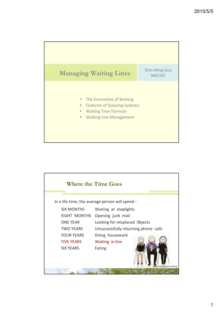
2015/5/5 Shin ‐ Ming Guo Managing Waiting Lines NKFUST • The Economies of Waiting • Features of Queuing Systems • Waiting Time Formula • Waiting Line Management Where the Time Goes In a life time, the average person will spend ‐‐ SIX MONTHS Waiting at stoplights EIGHT MONTHS Opening junk mail ONE YEAR Looking for misplaced 0bjects TWO YEARS Unsuccessfully returning phone calls FOUR YEARS Doing housework FIVE YEARS Waiting in line SIX YEARS Eating Japanese know waiting 1

2015/5/5 Waiting Realities • Inevitability of Waiting: Waiting results from variations in arrival times and service times • Economics of Waiting: High server utilization at the expense of customer waiting. Make waiting productive (salad bar) or profitable (drinking bar). The Economies of Waiting Cost Cost of Capacity Total Cost minimum Cost of Waiting Small Service Capacity Large Total cost per hour = Cost of capacity per hour + Cost of Waiting Time 4 2

2015/5/5 I. The Operation of a Typical Call Center Call center Answered Incoming Sales reps Calls calls processing Calls calls on Hold  At peak, 80% of calls dialed received a busy signal.  Customers getting through had to wait on average 10 min. . Blocked calls Abandoned calls (busy signal) (tired of waiting) Holding cost Lost throughput Cost of capacity $$$ Revenue $$$ Lost goodwill Cost per customer Lost throughput (abandoned) 5 A “Perfect or Somewhat Odd” Call Center Arrival Service Caller Time Time 1 0 4 2 5 4 3 10 4 4 15 4 5 20 4 6 25 4 7 30 4 8 35 4 9 40 4 10 45 4 11 50 4 12 55 4 7:00 7:10 7:20 7:30 7:40 7:50 8:00 6 3

2015/5/5 A More Realistic Service Process caller 1 caller 3 caller 5 caller 7 caller 9 caller 11 Service Caller Arrival Time Time caller 2 caller 4 caller 6 caller 8 caller 10 caller 12 1 0 5 2 7 6 Time 3 9 7 7:00 7:10 7:20 7:30 7:40 7:50 8:00 4 12 6 5 18 5 3 6 22 2 Number of cases 7 25 4 2 8 30 3 9 36 4 1 10 45 2 11 51 2 0 2 min. 3 min. 4 min. 5 min. 6 min. 7 min. 12 55 3 Service times 7 Variability Leads to Waiting Time Arrival Service Caller Time Time 1 0 5 Service time 2 7 6 3 9 7 4 12 6 5 18 5 Wait time 6 22 2 7 25 4 8 30 3 9 36 4 7:00 7:10 7:20 7:30 7:40 7:50 8:00 10 45 2 5 11 51 2 4 12 55 3 3 Inventory (callers on line) 2 1 0 8 7:00 7:10 7:20 7:30 7:40 7:50 8:00 4

2015/5/5 Ignoring Variability Leads to Over-Confidence Random arrivals and varying demands are common in services. In the presence of variability, one cannot estimate the process performance based on averages. Q: Why does variability not average out over time? A: You cannot inventory services — Capacity can never run ahead of demand. 9 Variability: Where does it come from? Tasks • Inherent variation • Lack of SOPs • Quality (scrap / rework) Processing Buffer Input • Unpredicted Volume swings Resources • Random arrivals • Breakdowns / Maintenance (randomness is the rule, • Operator absence not the exception) • Set ‐ up times • Incoming quality • Product Mix 10 5

2015/5/5 II. Essential Features of Queuing Systems Renege Arrival Queue Departure process discipline Service Calling Queue process population configuration Balk No future need for service 11 Calling Population 12 6

2015/5/5 Customer Arrival Process Arrival Arrival process process Static Dynamic Random arrival Random arrival Customer ‐ Random Facility ‐ exercised rate varying rate varying arrivals with controlled control constant rate with time with time Accept/Reject Price Appointments Reneging Balking Analyzing an Arrival Process Arrival Call Interarrival Time Time, AT i Call 1 Call 2 Call 3 Call 4 Call 5 Call 6 Call 7 IA i =AT i+1 -AT i 1 6:00:29 00:23 2 6:00:52 01:24 3 6:02:16 00:34 4 6:02:50 6:00 6:01 6:02 6:03 6:04 6:05 6:06 Time 02:24 5 6:05:14 00:36 6 6:05:50 IA 1 IA 2 IA 3 IA 4 IA 5 IA 6 00:38 7 6:06:28 standard deviation   2 CV Coefficien t of Variation a mean 14 7

2015/5/5 Distribution of Caller Inter-arrival Times Random (Poisson) arrivals  Customers arriving independently from each other follow exponential inter ‐ arrival times.     t f ( t ) e 1/  = average inter ‐ arrival time 2   = arrival rate CV 1 a Temporal Variation in Arrival Rates An arrival process is not stationary if the average number of arrivals in any given time interval is not fixed over the entire time period. 8

2015/5/5 Queue Configuration Multiple Queues vs. Single Queue Multiple Queues ? Single queue Take a Number 3 4 2 8 6 10 12 7 11 9 5 Enter 18 9

2015/5/5 Queue Discipline Queue discipline Static Dynamic (FCFS rule) selection selection Selection based Selection based based on status based on status on individual on individual of queue of queue customer attributes customer attributes Number of Processing time customers Round robin Priority Preemptive of customers waiting (SPT rule) Priority Rules in Waiting Time Systems  First ‐ Come ‐ First ‐ Serve: easy to implement + perceived fairness  Shortest Processing Time Rule: Minimizes average waiting time  Sequence based on importance: emergency or profitable customers A: 9 minutes B: 10 minutes C: 4 minutes D: 8 minutes A C 9 min. B 4 min. D 13 min. 19 min. C A 23 min. D 21 min. B Total wait time: 4+13+21=38 min Total wait time: 9+19+23=51min 20 10

2015/5/5 Service Process and Customer Involvement 21 Histograms of Service Times 1/ μ = mean service time μ = service rate  2  CV s  1 22 11

2015/5/5 III. Single Server Model: M/G/1  1. Mean arrival rate:  2. Mean service rate:    3. Mean number in service (utilization): long time  averages     2 2 2  4. Mean number of customers in queue: L   q 2 ( 1 )    5. Mean number of customers in the system: L L s q 1  6. Mean time in system: W L  s s 1 1    7. Mean time in queue: W L W   q q s Reducing Variability to Reduce Waiting   2 2 1 CV CV    a s W    q 1 2 Service time factor Utilization factor Variability factor Reduce Arrival Variability • appointment/reservation: how to handle late arrivals or no ‐ shows • encourage customers to avoid peak hours. Reduce Service Time Variability • training and technology • limit service selection • reduce customer involvement 24 12

2015/5/5 Multiple, Parallel Resources with One Queue number in service number waiting L q departure arrival Entry to system Begin Service Departure Time in queue W q Service Time 1/ μ Time in system W s =W q + 1/ μ 25 Waiting Time for Multiple, Parallel Resources Under the assumption that  arrival rate    Utilizatio n 1   service rate m we approximate the average waiting time as          2 ( m 1 ) 1 2 2 mean service time utilizatio n CV CV          a s Time in queue        m 1 utilizatio n  2    26 13

2015/5/5 The Power of Pooling Independent Resources 70.00 2x(m=1) m=1 60.00 Waiting Time W q 50.00 40.00 m=2 30.00 20.00 m=5 10.00 m=10 0.00 60% 65% 70% 75% 80% 85% 90% 95% Utilization Pooling benefits are lower if queues are not truly independent Pooled Resources (m=2) 27 Staffing over the Course of a Day Number of customers Number of Per 15 minutes CSRs 160 160 17 16 140 140 15 14 120 120 13 12 100 100 11 10 80 80 9 8 60 60 7 6 40 40 5 4 20 20 3 2 0 0 1 Time 0:15 0:15 2:00 2:00 3:45 3:45 5:30 5:30 7:15 7:15 9:00 9:00 10:45 10:45 12:30 12:30 14:15 14:15 16:00 16:00 17:45 17:45 19:30 19:30 21:15 21:15 23:00 23:00 28 14

2015/5/5 More on Reducing Wait Times  Appointment (no show?)  Segment customers (pay more)  Encourage customers to come during the slack periods  Provide limited service or self ‐ service  Provide 24x7 service or internet access  Flexible servers and flexible work hours  Technology: bar ‐ code, OCR, RFID (ETC) , Fast Lane, customer database 29 IV. Waiting Times & Customer Satisfaction Reducing average waiting time does not guarantee customer satisfaction. A small percentage of customers may experience long waits and complain bitterly. Solution: service guarantee and/or service recovery 30 15

2015/5/5 Service Levels in Waiting Systems 1 90% of calls had to wait 25 Fraction of Waiting times for those customers who 0.8 seconds or less customers who do not get served immediately have to wait x 0.6 seconds or less Fraction of customers who get 0.4 served without waiting at all 0.2 Waiting time [seconds] 0 TWT 0 50 100 150 200 Target Wait Time (TWT) depends on your market position and the importance of incoming calls for your business Service Level = Probability{Waiting Time  TWT} 31 Psychology of Waiting • That Old Empty Feeling: Unoccupied time goes slowly • A Foot in the Door: Pre ‐ service waits seem longer that in ‐ service waits • The Light at the End of the Tunnel: Reduce anxiety with attention • Excuse Me, But I Was First: Social justice with FCFS queue discipline • They Also Serve, Who Sit and Wait: Avoids idle service capacity 16